The Zero-Sum Fallacy
In life, your win is not my loss. This is contrary to what used to happen when we were hunter-gatherers, fighting for a limited quantity of meat or in the sporting world, where there is only one crown at the end of a competition. And changing this hard-wired ‘wisdom of zero-sum’ requires conscious training.
The Double ‘Thank You’ Moment
In his essay, The Double ‘Thank You’ Moment, John Stossel uses the example of buying a coffee. After paying a dollar, the clerk says, “Thank you,” and you also respond with a “thank you.” Why?
“Because you want the coffee more than the buck, and the store wants the buck more than the coffee. Both of you win.”
Except under coercion, transactions lead to positive-sum games; otherwise, the loser wouldn’t have traded.
A great example of our world of millions of double thank-you moments is apparent from how the global GDP has changed over the years.
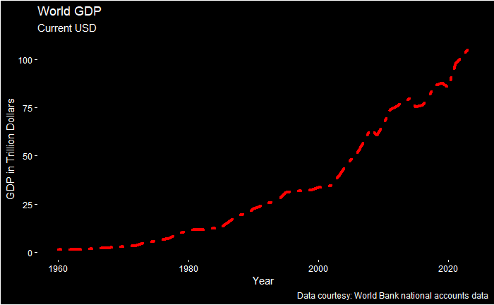
Notice that the shape of the curve is not flat but is exploding lately due to the exponential growth in transactions between people, countries and entities.
Inequality rises; poverty declines
One great tragedy that extends from the zero-sum fallacy is the confusion of wealth inequality with poverty. In a zero-sum world, one imagines that the rich getting richer must be at the expense of the poor! In reality, what matters is whether people are coming out of poverty or not.
Reference
GDP: World Bank Group
The Double ‘Thank You’ Moment: ABC news
The Zero-Sum Fallacy Read More »