Bread Sales
A bread salesman makes an average of 20 cakes; what is the chance he sells an even number of cakes?
Let’s assume the sales follow a Poisson distribution.
Reference
Fifty Challenging Problems In Probability: Frederick Mosteller
A bread salesman makes an average of 20 cakes; what is the chance he sells an even number of cakes?
Let’s assume the sales follow a Poisson distribution.
Fifty Challenging Problems In Probability: Frederick Mosteller
Adam finishes work at random times between 3 PM and 5 PM. His mother lives uptown, and his girlfriend lives downtown. After work, he goes to the metro station, catches the first train in either direction and has dinner with the person who lives on the side he reaches. His mother complains that his son came only two times in the last twenty working days, whereas Adam thought he was fair, with either party getting 50-50 chances. What’s really happening?
Suppose the metro on each side runs every 10 minutes, making it six times an hour: 3:00, 3:10, 3:20, etc. Let D represent the metro to downtown and U to uptown at x minutes after D.
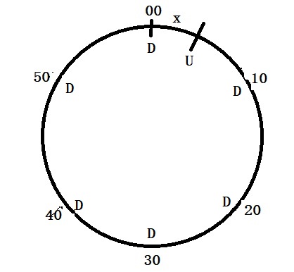
Since the mother saw him only twice in twenty days, the probability of Adam catching the uptown metro is 2/20 = 1/10, which must be equal to x/10. This implies x = 1. So the metro that goes uptown reaches its stop at 3:01, 3:11, 3:21, etc.
Fifty Challenging Problems In Probability: Frederick Mosteller
Mother vs Girlfriend Read More »
There are two urns: Urn 1 contains two red balls and one black ball, and Urn 2 has 101 red balls and 100 black balls. Two balls can be taken from one of the urns at random. The task is to correctly identify the urn from which the balls have been collected. After the first draw, you can decide whether to replace the ball. What will be your strategy?
If the first ball is red, the remaining balls in Urn 1 are one red and one black, and in Urn 2, 100 red and 100 black. That means the probability of drawing any colour is equal (0.5) from each urn. As this can’t help deciding the correct urn, return the red ball and pull the second ball.
If the first ball is black, the remaining balls in Urn 1 are two reds and zero black, and in Urn 2 are 101 red and 99 black. In such a case, do not replace the ball, as the probabilities of red and black are different in each urn, which helps identify the urn better.
Let’s apply Jensen’s Inequality to the housing market. It concerns default rates on housing loans with the housing prices. When the housing prices are high, the defaults reduce; when the prices are lower, defaults increase but not in the same magnitude. Here is a fictitious plot of % of bank profit vs % change in housing price.
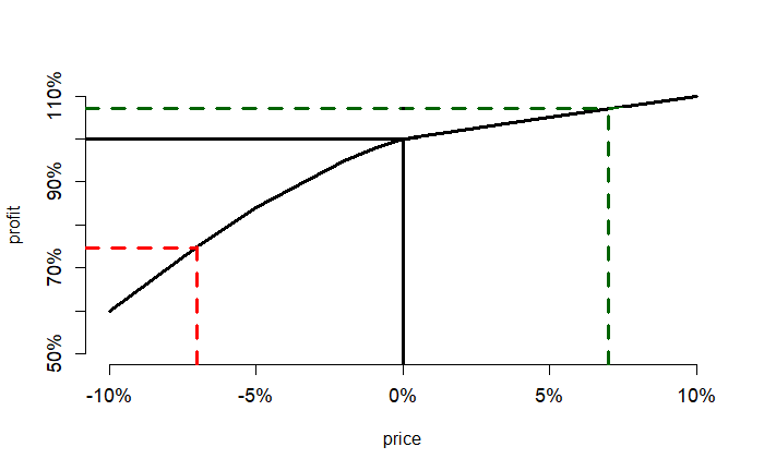
A 7% increase in house price increases the bank’s profit by about 7%, whereas an equivalent decrease in price leads to about a 25% drop in profit!
Jensen’s Inequality and Banking Collapse Read More »
Before analysing inequality, let’s develop an intuition. Suppose the profit from sales of an object moves the following way with the price.
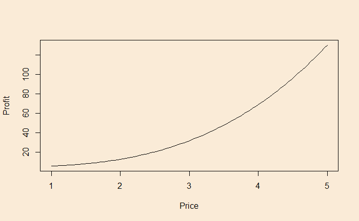
The price can be 2, 3, or 4 in a given year with equal probabilities. What is the average profit?
The mathematical function that presents the above behaviour is x3 + 5. Suppose the price values (x) 2, 3, and 4 can occur equally likely. This means the average price value is (2+3+4)/3 = 3. The profit at x = 3 is 33+5 = 32.
Let’s estimate the profit at each x value and then take the average.
at x = 2, profit = 23+5 = 13
at x = 3, profit = 33+5 = 32
at x = 4, profit = 43+5 = 69
Average is (13+32+69)/3 = 38
This is Jensen’s inequality, which says that the average (expected values) of inputs do not lead to average output if the function is non-linear. Depending on the shape of the non-linearity, it can under-estimate or over-estimate.
Jensen’s Inequality Read More »
An aircraft has 200 seats. The airline knows that, on average, 5% of the people who have purchased the ticket don’t show up. What is the maximum number of tickets they can sell to manage the probability that more than 200 passengers will show up at 10%?
The number of people who do not show up (X) will follow a binomial distribution with a probability of success of 5%, X ~ Bin(200+X, 0.05). Since X is unknown, we first use the qbinom function on 200 to get an approximate solution.
qbinom(0.1, 200, prob = 0.05, lower.tail = TRUE) 6Now, we use 200+6 in the equation.
qbinom(0.1, 206, prob = 0.05, lower.tail = TRUE)6We have seen how the constant pi is estimated as a fraction of randomly ‘hitting darts’ on a circle inscribed inside a square. Here, we see how the same is done by numerically integrating a unit circle between -1 and 1.
The first part is to create the functions for the circle.
f <- function(x)  sqrt(1-x^2)
f1 <- function(x)  -sqrt(1-x^2)
You can check it by plotting the functions using the R command ‘curve’ and shading the area using the ‘shade’ function from the library, ‘DescTools’.
min <- -1
max <- 1
par(bg = "white", pty = "s")
curve(f, from = min, to = max, ylim = c(-1,1))
curve(f1, from = min, to = max, add = TRUE)

Shade(f, breaks = c(min,max), col = "darkgreen", density = 20)
Shade(f1, breaks = c(min,max), col = "darkgreen", density = 20)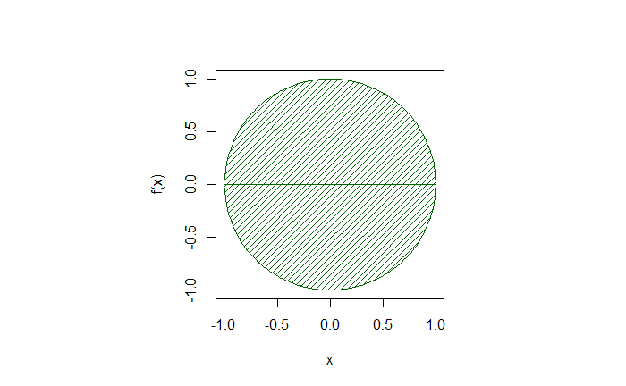
Evaluate the function between the limits to get the area.
points <- seq(min, max, by = 0.000001)
(max-min)*mean(f(points)) - (max-min)*mean(f1(points))3.141591Another example is the area of the normal distribution between -1.96 and +1.96 for the well-known 95% confidence interval.
f <- function(x)  dnorm(x)
curve(f, from = -5, to = 5)

min <- -1.96
max <- 1.96
Shade(f, breaks = c(min, max), col = "darkgreen", density = 20)

points <- seq(min, max, by = 0.00001)
(max-min)*mean(f(points))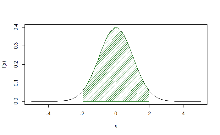
0.9500024Integrating Circle for Pi Read More »
A car hire firm typically receives an average of 3 hiring requests per day. What is the probability it gets at most two hiring requests for exactly 3 days a week?
The first part of the problem (getting at most 2 requests in a day) can be solved using the Poisson probability model. It involves a random variable, X, and it takes positive values. All we know is an expected value (average value), lambda. The probability is expressed as:
![]()
Now, substitute lambda = 3 and s for at most 2 requests, i.e., the chance of 0 requests + 1 request + 2 requests.

This can be easily estimated using the R code:
ppois(2, 3, lower.tail = TRUE)This is the daily probability for at most 2 car hire requests. For estimating the probability of 3 exact such days in a week, we use the binomial model.

Or the R code.
dbinom(3, 7, prob = ppois(2, 3, lower.tail = TRUE))The Poisson Cars and Binomial Hires Read More »
In their paper ‘Methods for Studying Coincidences, ‘ Diaconis and Mosteller propose the law of truly large numbers, which states that almost any outrageous event is bound to occur with a large enough number of independent samples!
Imagine an event that happens with a probability of 0.1% or 0.001. Therefore, the chance that it doesn’t happen is 0.999. If you carry out 100 independent trials, the probability of this not occurring is 0.999100 = 0.90. In other words, there is a 1-0.9 = 0.1 or 10% chance of occurrence. The following is the plot of this from 1 to 10,000 trials.
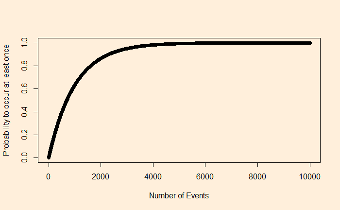
You can see that beyond, say, 5000 independent trials, this rare event is sure to occur at least once.
Law of Truly Large Numbers Read More »
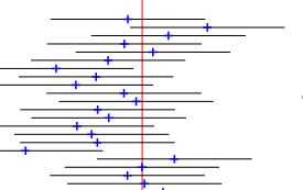
Confidence interval is a frequentist’s way of communicating the range of values within which the actual (population) parameter sits. A confidence interval of 90% implies that if you do 20 random samples from the same target population and with the same sample size, 18 of the confidence intervals cover the true population mean. This is the frequentist’s view, and the parameter is fixed.
On the other hand, the Bayesian does not have a concept of a fixed parameter and is happy to accept it as an unknown quantity. Instead, she gives a probability distribution to the expected outcome. The range of values (the interval) of the probability distribution (plausibility) is the credibility interval. In a 90% credible interval, the portion of the (posterior) distributions between the two intervals will cover 90% of the area.
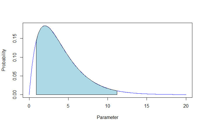
For example, in the following posterior distribution, there is a 90% plausibility that the parameter lies between 0.9 and 11.2; the shaded area = 0.9.
Confidence Interval vs Credible Interval Read More »