A survey revealed the following information on the prevalence of eye disease. Check if the difference in prevalence is statistically significant.
Residence
Eye Disease
Total
Yes
No
Rural
24
276
300
Urban
15
485
500
n1: sample size of population 1 = 300 n2: sample size of population 2 = 500 p1: sample proportion for population 1 = 24/300 p2: sample proportion for population 2 = 15/500
Critical z = 1.96 at a 5% confidence interval. Therefore, z = 2.87 > critical z; the difference in prevalence of eye disease between urban and rural is significant.
The Enigma machine was an electromechanical device built by the Germans in World War II to mechanise encryption. The device was about the size of a typewriter and had two sets of letters on a keyboard and a lampboard. The message got encrypted letter by letter.
The Enigma machine was a large circuit. It had the following components.
Rotors 1, 2, and 3. They connected the cris-cross wires from one letter to another. But these three rotors are selected from a total of five.
The reflector connected 26 letters into 13 pairs.
The plugboard connected some letters into pairs, and some were left unconnected. In one version, it connected 20 letters into ten pairs and left six unpaired.
So what are the total possibilities?
1) 3 chose from 5 (and order matters) => 5!/2! = 60. 2) Three rotors with 26 letters available => 26 x 26 x 26 possibilities 3) 10 pairs from 26 possible letters => 26!/6!10!210. 210 comes because a pair AB is indistinguishable from BA, and there were 10 such combinations.
Multiply all three, and you get the possible ways to set the enigma machine! That equals 1.589626e+20.
We will use utility curves to illustrate three different kinds of risk preferences. They are:
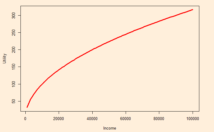
Risk-averse
Here is a person who has the diminishing utility of marginal wealth. I.e., the extra dollar additional income from 10,000 to 10,001 brings a lesser increase in happiness to her than going from 100 to 101.
Notice the probabilistic (expected) utility line (blue) is below the certainty (brown).
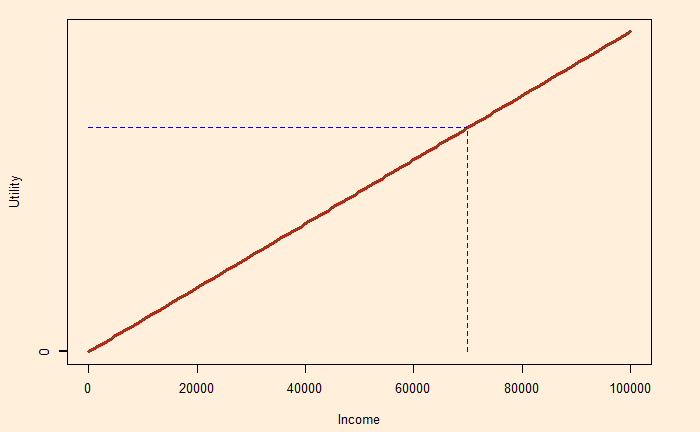
Risk neutral
This person shows constant marginal utility. The person has the same happiness with a 1 dollar salary rise whether her current is at 10,000 or 100,000.
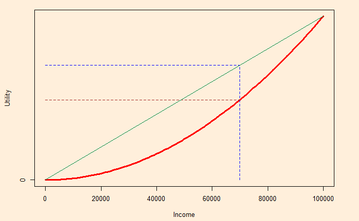
Risk lover
Imagine someone needs 100,000 for a major surgery to save her life. Smaller numbers don’t make much sense to her, and she is willing to gamble for a larger prize. She has increasing marginal utility.
Unsurprisingly, the expected utility line (blue) is above the certainty (brown).
Think about this game. There is a 1 in 1000 chance of winning a prize of 1 billion. The price of the ticket is $1. Will you take the gamble? Definitely, it is a good deal to buy the ticket. You only lose a dollar but get a chance to win a billion (expected value of a million).
Pascal used a similar argument to state that belief in god was a better deal than not doing so. He argues: Proposition 1: God exists Proposition 2: God doesn’t exist If god exists and you believe, the payoff is infinitely good If god exists and you don’t believe, the payoff is much worse On the other hand, if god doesn’t exist, regardless of whether you believe in it or not, the payoffs (positive and negative) are finite. So, he argues, believing is a better deal.
God exists (G)
God does not exist (¬G)
Belief (B)
infinite gain
finite loss
Disbelief (¬B)
infinite loss
finite gain
Based on the payoff matrix, there is only one rational (!) decision: choose B.
A country has two teams of weightlifters; in one, 80% use steroids regularly, and in the other, only 20% use them. The head coach flips a coin and selects the team for the international meet. At the venue, if one lifter was selected at random for the drug test and found positive, what is the probability that the team is the steroid one?
We will use the base form of Bayes’ theorem – the relationship between conditional and joint probabilities.
P(S/T) = P(S & T) / P(T) S – it is a steroid team T – tested member used steroid C – it is a clean team
P(S & T) = P(S) x P(T|S) = 0.5 (coin toss) x 0.8 (chance of using steroids, given he is from the steroid team) = 0.4 P(T) = P(S) x P(T|S) + P(C) x P(T|C) = 0.5 x 0.8 + 0.5 x 0.2 = 0.5 P(S/T) = 0.4/0.5 = 0.8
The probability that the team is the steroid one is 80%
Cap and trade is amethod of regulatory intervention to reduce carbon emissions. Here, the system sets a maximum value for the emissions (cap). It also provides allowances, in emission permits, to firms to cover each unit of CO2 (or any other pollutant) produced. The company can redeem one for every emission unit or trade it to another party, who can then use it.
The regulator can issue permits to the firm in two ways. It can give away permits for free (based on some criteria) or auction them. Allocating permits based on past emissions is called grandfathering.
Mathematically, economists proved that the fee of permits has no impact on the price of the product. If p is the price, q is the output, c(q) is the cost of production, pp is the permit cost, and A is the free permit.
1) For zero free permit profit = p q – C(q) – ppq The firm maximises its profit with respect to quantity, d(profit)/dq = p – C'(q) – pp = 0 price of the product, p = C'(q) + pp
2) For ‘A’ free permits profit = p q – C(q) – (ppq – A) The firm maximises its profit with respect to quantity, d(profit)/dq = p – C'(q) – pp = 0; A is a constant and its derivative is zero. price of the product, p = C'(q) + pp
So, in both cases, the product’s price is the marginal cost + the price of the permit. The auction, at least, gives the government some money that can be used to support the people who are the worst affected by the price rise.
The story of Martin and Big Fish, taken from ‘An Introduction to Probability and Inductive Logic’ by Hacking, is about risk and insurance.
Marting sells clothes on the streets. His sales are typically about $300 and cost $100. Since he is not registered as a vendor at that location, he gets tickets from the authorities for illegal sales. The fine is $100, and he estimates that they happen about two times on his 5-day week.
The daily expected value of his work is: (2/5) x (300 – 100 -100) + (3/5) x (300 – 100) = $160.
Now, Big Fish finds Martin offers his stall at a daily rent of $50. Martin’s new return can become 300 – 100 – 50 = 150. Should he agree with this?
It is a trade-off for Martin; his profits come down, but he runs no risk now. It is possible that the number of raids increase in future. The same can happen with the fine amount. By paying the additional $10, he replaced the risk with certainty.
Reference
An Introduction to Probability and Interactive Logic by Ian Hacking
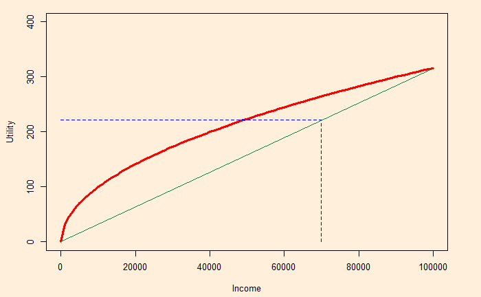
We have seen how risk-averse and risk-taking behave differently given options to take a certain $70,000 or a gamble with a 70% chance of winning $100,000. The former will take $70,000, and the latter will try the luck of winning $100,000. Remember, the expected value of both choices remains the same – $70,000. We have also seen that the utility of that money increases as the square root of the income (decreasing utility rate).
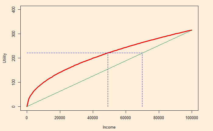
Also, using this example, we will work out the value of guarantees (insurance) for the risk-averse. The utility of the expected value is graphically represented as:
The vertical line touches the X-axis at 0.7 x 100,000 = 70,000, and the expected utility (not the guaranteed) is where the horizontal line touches the Y-axis. We have estimated this value in the previous post as 221.36.
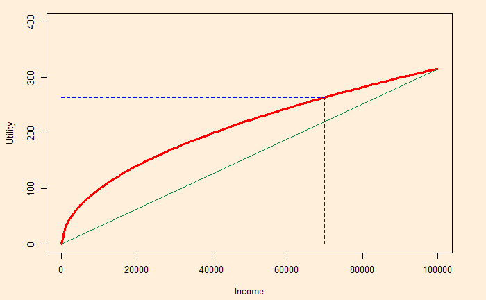
When the income is guaranteed (at 70,000), the corresponding utility becomes:
This guaranteed utility is 264.58, which the risk-averse is perfectly happy to accept. Note that the risk-lover is aiming for the full utility. (Although, in the process, she might end up with nothing!)
Insurance
The insurer can guarantee $70,000 at a fee. It is because, whereas it may have to give the individual $70,000, the insurance company knows that if several people gamble, at the end of the day, they will get $70,000. In other words, the expected value exists for the entity that oversees hundreds of gambles and not for the individual who only sees 0 or 100,000. And the fees become the profit for the company.
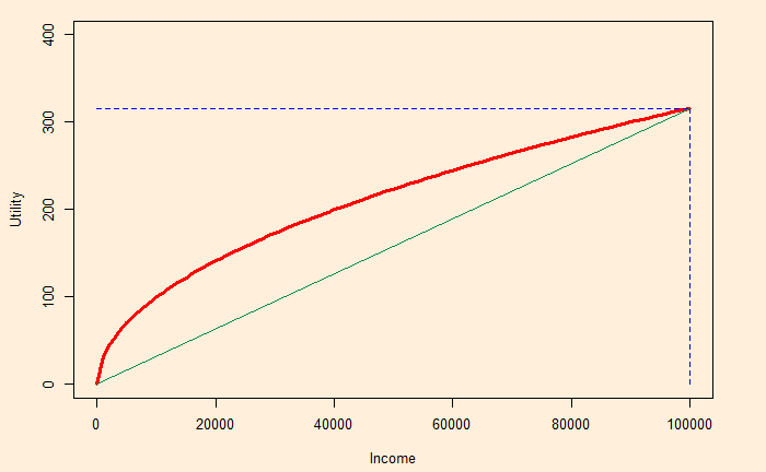
Look at how much income the gamble is worth (with certainty). It is the point at which the black dotted line hits the X-axis in the representation below:
It is about 49,000 in our example. The insurer absorbs it and promises 70,000. The individual and insurer may split the difference (70,000 – 49,000 = 21,000). Say, in one case, the insurer charges 5,000 as the fee, leaving the person with 65,000, equivalent to a utility of $253.
Let’s go one step further in the expected utility story. Here, we use the same utility function, I1/2, but a different probability of success. This time, the gamble has a 70% chance to get 100,000 vs. 30% chance to lose everything. The expected value is 0.7 x 100,000 + 0.3 x 0 = 70,000
The expected utility is: 0.7 x(100,000)1/2 + 0.3 x 0 = 221.36
Imagine someone guarantees the expected value (70,000). The utility of this amount is: 70,0001/2 = 264.58
Surely, the second person, who is guaranteed the value, is happier. In other words, the risk is removed, or certainty is added in the second case. So, the question is: what is the price of that ‘insurance’?
We have seen what expected utility is and how it’s different from the expected value. Suppose Amanda earns 100,000 dollars a year and has a 1% chance of getting sick. The cost of sickness is 50,000 dollars (on medical bills). Amanda’s utility function is:
U = I1/2; where I is the income.
What is her maximum willingness to pay for insurance that covers 50,000 dollars in medical bills?
The maximum willingness to pay is the price, at which she is indifferent between buying the insurance and not. Therefore,
Expected utility with insurance = Expected utility without insurance. (100,000 – P)1/2 = 0.99 x (100,000)1/2 + 0.01 x (100,000 – 50,000)1/2 P = 100,000 – [(0.99 x (100,000)1/2 + 0.01 x (100,000 – 50,000)1/2)]2 P = $585