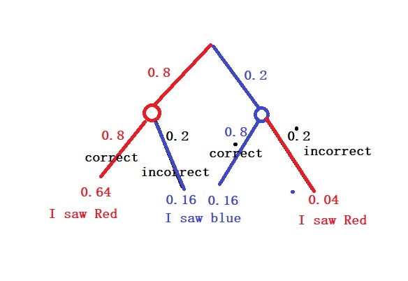
November 2023

The Guessing Game

A student is attempting an exam with multiple-choice questions with four options for each question. She knows the correct answer for half of the questions and plans to guess the other half.

If a given response is correct, what is the probability that she guessed that answer?

Let P(G) be the probability for her to guess an answer, which we know is half or 1/2. P(G’), the probability she did not assume (because she knows the answer), is 1 – P(G) = 1/2. If she guesses an option, the chance that it is correct is P(C|G) = 1/4 (one in four). On the other hand, P(C|G’), where she did not guess, the probability for it to be correct is 1.

The required probability is P(G|C), or the chance that she guessed, given the correct answer.

\\ P(G|C) = \frac{P(C|G)*P(G)}{P(C|G)*P(G) + P(C|G')*P(G')} \\\\ = \frac{1/4 * 1/2}{1/4 * 1/2 + 1 * 1/2} = 1/5

20% chance.

The Guessing Game Read More »

Card Shuffle

How many cards are expected to retain the original, i.e., the place before the shuffle, position in a well-shuffled deck of cards?

Let X1 be the event where the first card retains position one after the shuffle. We give a value of 1 if it gets the right spot and 0 otherwise. A shuffled card can occupy any of the 52 positions; therefore, the probability of getting any place (including the first) is 1/52. The expected value for X1 becomes:

E(X1) = 1 x (1/52) + 0 x (51/52) = 1/52

It’s easy to notice that E(X2) also follow the same logic and becomes 1/52, etc.

The expected number for each card to stay in the same spot is:

E(X1 + X2 + X3 … X52) = E(X1) + E(X2) + E(X3) + … E(52) = 52 x (1/52) = 1

You can see that this is true for any number of cards from 1.

Card Shuffle Read More »

Average Temperature in Jakarta

The average temperature in June in Jakarta is 32 oC with a standard deviation of 5 oC. If the temperature in June follows a normal distribution:

  1. What is the probability of observing higher than 40 oC on a random June day in Jakarta?
1 - pnorm(40, mean = 32, sd = 5)
0.0548

Let’s estimate the same thing using the ‘pnormGC’ of ‘tigerstats’ package.

pnormGC(40, mean = 32, region = "above", sd= 5, graph = TRUE)

2. How cold are the coldest 10% days in June in Jakarta?

 qnorm(0.10, mean = 32, sd = 5)
25.59224
 pnormGC(25.59224, mean = 32, region = "below", sd= 5, graph = TRUE)

Average Temperature in Jakarta Read More »

The story about 2% fat milk

What is a 2% fat milk? Let’s first look at what it contains:

240 ml milk weighs around 245 g. So, the percentage weight of milk is 5 g / 245 g = 0.02 or 2%.
The milk carries a total of 130 calories, and out of these, the fat calorie is 45., which is 45/130 = 0.346 = 35%

So, this is 35% milk as well! But the producer will likely stick with the 2% narrative as it sounds healthier!

The story about 2% fat milk Read More »

Amy’s Job

Amy got short-listed for three job interviews. The total number of candidates appearing for the three jobs are 5, 3 and 4. Assuming all the candidates are equally competent, what is Amy’s chance of getting at least one job?

Step 1: Assume probabilities are independent. 

Step 2: Estimate the probabilities of getting rejected in each job. i.e., 1 – 1/5 = 4/5, 1 – 1/3 = 2/3, and 1 – 1/4 = 3/4. 

Step 3: Calculate the joint probability of getting left in all jobs. (4/5)x(2/3)x(3/4) = 0.4

Step 4: Probability of getting at least one job = 1 – probability of getting rejected from all jobs, i.e., 1- 0.4 = 0.6

Amy’s Job Read More »

One-Sample Poisson: Car Breakdown

A car model breaks down on average 1.5 times a year. The company has developed a fix that claims to have reduced the issue. Alby randomly selects ten cars of the new model and finds eight of them break down in the first year. Did the fix work? Use a significance level (alpha) of 5%.

Since the subject represents counts (car breakdowns) that occur at random, we will use the Poisson Hypothesis testing here.

The null hypothesis, H0 = the average failure rate (lambda) of the new car = 1.5 (same as old)
The alternate hypothesis, HA = the average failure rate (lambda) of the new car < 1.5 (failure reduced)

The R code has the following format: poisson.test(total count, duration, hypothesized rate, region of the alternative)

poisson.test(8, 10, 1.5, alternative = "less")
	Exact Poisson test

data:  8 time base: 10
number of events = 8, time base = 10, p-value = 0.03745
alternative hypothesis: true event rate is less than 1.5
95 percent confidence interval:
 0.000000 1.443465
sample estimates:
event rate 
       0.8 

Since we used the p-value as the criterion and it is less than the significance level (0.05), we reject the null hypothesis in favour of the notion that the fault has been reduced.

Reference

Hypothesis Testing with the Poisson Distribution

One-Sample Poisson: Car Breakdown Read More »

Two-Sample Poisson Test

Two batches of products have come from a factory with the following defect counts. Find out whether one batch made fewer defects than the other batch.

Total number of samples = 30 each
Rate occurrences = 107/30 = 3.56 and 161/30 = 5.36

poisson.test(c(107, 161), c(30, 30))
Comparison of Poisson rates

data:  c(sum(r_data$Supplier.1), sum(r_data$Supplier.2)) time base: c(30, 30)
count1 = 107, expected count1 = 134, p-value = 0.001166
alternative hypothesis: true rate ratio is not equal to 1
95 percent confidence interval:
 0.5155166 0.8539201
sample estimates:
rate ratio 
 0.6645963 

There is a difference between the two batches of samples.

Comparing Hypothesis Tests for Continuous, Binary, and Count Data: Statistics by Jim

Two-Sample Poisson Test Read More »

One-Sample Poisson Test

The city council claims their recent road safety campaign has reduced the daily accident rate. The following are the daily data collected over 20 days. The mean rate before the campaign was 5.

4, 6, 4, 1, 1, 5, 5, 6, 3, 5, 1, 8, 3, 2, 5, 7, 5, 2, 3, 4

The first thing to realise here is that the number of accidents is entirely random, although it may revolve around a mean (rate). Therefore, the hypothesis tests based on normal distribution, such as t.test, are not applicable here. We use the Poisson test on such occasions.

poisson.test(80, 20, 5, alternative = "less")

Here, 80 is the sum of the counts, and 20 is the total duration (days) over which the samples were collected.

	Exact Poisson test

data:  sum(x) time base: 20
number of events = 80, time base = 20, p-value = 0.02265
alternative hypothesis: true event rate is less than 5
95 percent confidence interval:
 0.000000 4.817502
sample estimates:
event rate 

The p-value = 0.022, and we reject the null hypothesis, H0 (that the event rates are equal), at a significance level of 5%.

One-Sample Poisson Test Read More »