We have seen how the constant pi is estimated as a fraction of randomly ‘hitting darts’ on a circle inscribed inside a square. Here, we see how the same is done by numerically integrating a unit circle between -1 and 1.
The first part is to create the functions for the circle.
f <- function(x)  sqrt(1-x^2)
f1 <- function(x)  -sqrt(1-x^2)
You can check it by plotting the functions using the R command ‘curve’ and shading the area using the ‘shade’ function from the library, ‘DescTools’.
min <- -1
max <- 1
par(bg = "white", pty = "s")
curve(f, from = min, to = max, ylim = c(-1,1))
curve(f1, from = min, to = max, add = TRUE)

Shade(f, breaks = c(min,max), col = "darkgreen", density = 20)
Shade(f1, breaks = c(min,max), col = "darkgreen", density = 20)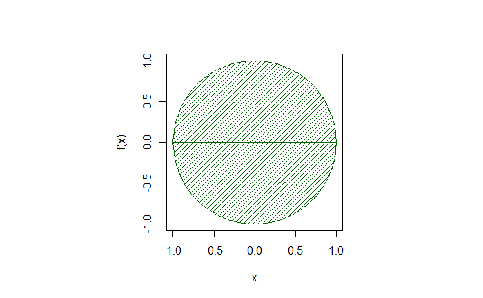
Evaluate the function between the limits to get the area.
points <- seq(min, max, by = 0.000001)
(max-min)*mean(f(points)) - (max-min)*mean(f1(points))3.141591Another example is the area of the normal distribution between -1.96 and +1.96 for the well-known 95% confidence interval.
f <- function(x)  dnorm(x)
curve(f, from = -5, to = 5)

min <- -1.96
max <- 1.96
Shade(f, breaks = c(min, max), col = "darkgreen", density = 20)

points <- seq(min, max, by = 0.00001)
(max-min)*mean(f(points))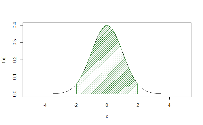
0.9500024
