June 2023

Shark Attack and Randomness – A Case for Changepoint?

We have seen randomness explaining the ‘trends’ in shark attacks in South Africa. The next one is Australia. Here is the scatter from 1980-2023.

Scatter plot

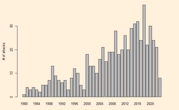
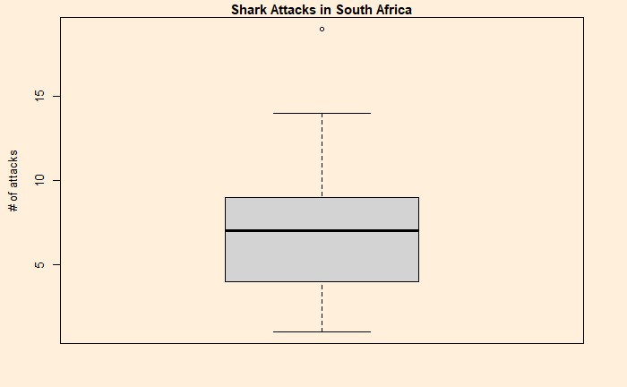
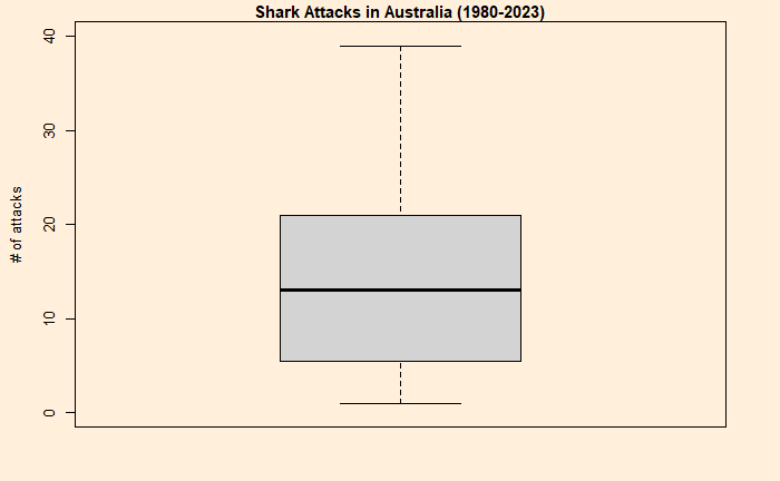
It looks like two different clusters or trends, as apparent from the plot, and the change point may have happened sometime in 2000. Another way of visualising the statistical summary is to build boxplots.

Boxplot summary

A t-test is handy here to test the hypothesis (that the two trends are just by chance or not).

T-test

Aus_before <- inv_afr$AUS[which(inv_afr$Year < 2000)]
Aus_after <- inv_afr$AUS[which(inv_afr$Year > 1999)]
t.test(Aus_before, Aus_after, var.equal = TRUE)
	Two Sample t-test

data:  Aus_before and Aus_after
t = -8.6826, df = 42, p-value = 6.378e-11
alternative hypothesis: true difference in means is not equal to 0
95 percent confidence interval:
 -19.28749 -12.01251
sample estimates:
mean of x mean of y 
     5.85     21.50 

Comparison with South Africa

	Two Sample t-test

data:  SA_before and SA_after
t = 1.2881, df = 42, p-value = 0.2048
alternative hypothesis: true difference in means is not equal to 0
95 percent confidence interval:
 -0.8406907  3.8073574
sample estimates:
mean of x mean of y 
 7.900000  6.416667 

Unsurprisingly, the results show a p-value higher than the significant value (e.g., 0.05).

Shark Attack and Randomness – A Case for Changepoint? Read More »

Shark Attack and Randomness

People often quote shark attacks as examples for explaining randomness. For one, they have been sporadic. For example, here are statistics from South Africa.

Global Shark Attack – Worldmarising the Statistics.

The plot looks decent except for one outlier – 19 – in 1998.

One way to understand the pattern is to run a simulation assuming randomness and then compare the outcomes. Poisson distribution is best suited to make the check. Here is what we can do.

First, we plot the distribution of the actual data (in blue), followed by a comparison with the Poisson (in red).

Except for the outlier, the two plots are reasonably in agreement. Then, what about the shark attacks in Australia? That comes next.

Shark Attack and Randomness Read More »

Dice Polynomial

We have seen craps and how it is played based on the sum of two dice. And here is how the totals distribute. The question is: is there another way of throwing two dice (with another set of numbers on it) and playing the game of craps using the same rules.

Before finding the answer, let’s check how to represent a die. You can describe a die with this polynomial.

f(x) = x6 + x5 + x4 + x3 + x2 + x1

Rolling a pair of dice is nothing but multiplying this function with itself.

f(x) x f(x)= (x6 + x5 + x4 + x3 + x2 + x1) (x6 + x5 + x4 + x3 + x2 + x1)

x12 + 2x11 + 3x10 + 4x9 + 5x8 + 6x7 + 5x6 + 4x5 + 3x4 + 2x3 + x2

Check the table again; you will see from the coefficients and the exponents of the resulting polynomial that there is one way to roll a 12, two ways for 11 etc.

Dice Polynomial Read More »

Card Game – Optimal Decisions

Here is a game of cards. A and B have two cards each – one green and one red. If A shows green and B shows green, A wins 5 – 0. If A shows green and B shows red, A loses 2 – 3. If A shows red and B shows green, A loses 0 – 5. If A shows red and B shows red, A wins 5 – 0. Here is the representation of the rules.

Looking carefully at the rule, you can conclude that the game is in A’s favour. But can A guarantee the maximum score, and how?

Here is the payoff matrix in the game theory format.

Before getting into the proper formulation, let’s check what happens if A plays only green. A might get a few wins early on, but once B figures out, she will play only red and win by 1 (2-3). On the other hand, if A plays only red, B will play green and win 5 (0-5).

A mixes up

Let A mixes up the play at a probability PAG for green (1 – PAG for red). If she aims to provide no incentive for B to show either green or red,
The payoff for B showing green = Payoff for B showing red
0 x PAG + 5 x (1-PAG) = 3 x PAG + 0 x (1-PAG)
5 – 5 PAG = 3PAG
PAG = 5/8 = 0.625

B mixes up

Naturally, B may respond by mixing her game, PBG for green. Using the same argument from B’s standpoint
The payoff for A showing green = Payoff for A showing red
5 x PBG + 2 x (1-PBG) = 0 x PBG + 5 x (1-PBG)
5PBG + 2 – 2PBG = 5 – 5PBG
PBG = 3/8 = 0.375

Equilibrium outcome

At these rates (PAG, PBG), the expected outcome for A is:
(5/8)(3/8)(5) + (5/8)(5/8)(2) + (3/8)(3/8)(0) + (3/8)(5/8)5 = 3.125

And the expected outcome for B is:
(5/8)(3/8)(0) + (5/8)(5/8)(3) + (3/8)(3/8)(5) + (3/8)(5/8)0 = 1.875

Card Game – Optimal Decisions Read More »

Defective Shirts

This one is taken from a lecture by Eddie Woon, available online. Two friends, Ammie and Becky, make shirts. Ammie makes 20 shirts a day and has a defect rate of 2%. Becky is 50% faster but causes twice the defects. If they sell 30 shirts per day, what is the probability that the daily pack (received by the buyer) has two or fewer defects?

The first step is to calculate the defect probability.

P(D) = Proportion of shirt by Annie x Defect rate of Annie + Proportion of shirt by Becky x Defect rate of Becky
P(D) = (20/50)(2/100) + (30/50)(4/100) = 0.032.

Now, we apply the binomial equation to calculate the probability of having two or fewer defects inside the pack of 30- shirts.

the probability of s success in n rounds is
nCs x ps x q(n-s)

30C0 x 0.0320 x (1- 0.032)30 + 30C1 x 0.0321 x (1- 0.032)29 + 30C2 x 0.0322 x (1- 0.032)28 = 0.93 or 93%

The R code is

pbinom(2, 30, 0.032)

Binomial Probability: Eddie Woo

Defective Shirts Read More »

Coin-Toss Game – Misleading Averages

We have seen how a seemingly profitable game, because of its positive expected value and high average compounding rate, still leads to losses for the average player.

For example, in a simulation of 10000 people betting up to 50 times starting with $100, the number of them ending up with less than the initial amount is:

# Bets# that lost money
(out of 10,000)
205805
307057
507560

The original game implied an average gain of 15% per toss but at a certain probability of winning and losing. It assumed the individual was betting all the money she had earned so far in the subsequent bet. Here, we vary the amount per bet as a fraction of the total and then calculate the optimum fraction that yields profit to the median. But first, the misleading average wealth after 50 wagers, starting with $100.

It’s absurd to see how the gain rises exponentially. Then, we look at the median outcome for the individuals.

We notice there is an optimum strategy, somewhere close to 40%, that gives a modest, nonetheless positive return. Two such situations are illustrated based on how ten people performed after 25 games – the batch betted 100% money and the second person 30% each time.

Note that the Y-axis is in the log scale to resolve the variation better over a wide range.

Coin-Toss Game – Misleading Averages Read More »

Asymmetric Coin-Toss Game

Here is another coin-tossing game. If it lands on heads, your money increases by 80%, and if it’s tails, it reduces by 50%. The question is: will you play this game?

As always, let’s estimate the expected value of this game.
E =0.8 x 0.5 – 0.5 x 0.5 = 0.4 – 0.25 = 0.15 or a net gain of 15%. In other words, if I start with $100 and bet everything each time 20 times, on average, I end up getting 100 x 1.1520 = $1637.

Let 10,000 play this game and collect the average.

n_people <- 10000
n_bet <- 20
gain <- data.frame(matrix(NA, nrow = n_bet, ncol = n_people))
 
  for (m in 1:n_people) {
       bet1 <- 100
       money <- c(rep(0, n_bet))
       for (n in 1:n_bet) {
           bet2 <- bet1
           toss <- sample(c(0.8*bet2,-0.5*bet2), size = 1, replace = TRUE, prob = c(1/2,1/2))
           bet1 <- bet1 + toss
           money[n] <- bet1 
           gain[n,m] <- money[n]
       }
  }   
  gain$AVG <- apply(gain, 1, mean, na.rm=TRUE)

Yes, we get $1694.8 as the average of 10,000 people at the end of 20 rounds.

So, a no-brainer, huh? But before we make a decision, what is the median return from the game? In other words, what does the average person get: it’s 34.86!

gain$MED <- apply(gain, 1, median, na.rm=TRUE)

So, the average person systematically loses money.

Asymmetric Coin-Toss Game Read More »

Expected Value of Spin

There is a wheel with three values of 0, 1 and 2. Each occupies an equal area of the wheel. You play the game by spinning the wheel. If it lands on 1 or 2, you get the money and spin again. When it lands on 0, the game ends. What is the average value expected from this game?

There is a (1/3) chance the game ends with no money. There is a (2/3) chance that you get 1 or 2. So the expected value for game one is (2/3) x (3/2). For the second game, it is (2/3) x (2/3) x (3/2). So the total expected value is a sum of the following series.

(3/2) x [(2/3) + (2/3)^2 + (2/3)^3 + …]. The sum in the square bracket is 2; the product becomes (3/2) x (2) = 3.

Expected Value of Spin Read More »

Mtcars Dataset – Pair Plots

We continue with the mtcars dataset to illustrate a few more correlation plots – this time, the pair plots.

library(GGally)
ggpairs(car_data[,1:7])
  • The main diagonal represents the data distribution of the variable
  • The upper half diagonal represents the correlation coefficients
  • The lower half diagonal represents a scatter plot between pairs 
library(psych)
pairs.panels(car_data, lm = TRUE)

Mtcars Dataset – Pair Plots Read More »