November 2021

Vaccine Effectiveness and Incident Rates

I have shown you my estimates on vaccine effectiveness in Kerala in an earlier post. The plot is reproduced below.

You may have noticed that the effectiveness was steadily going upwards. Intrigued, it has prompted me to check what was going on with the other variables during the same period. One of them was the overall incident rate (shown below).

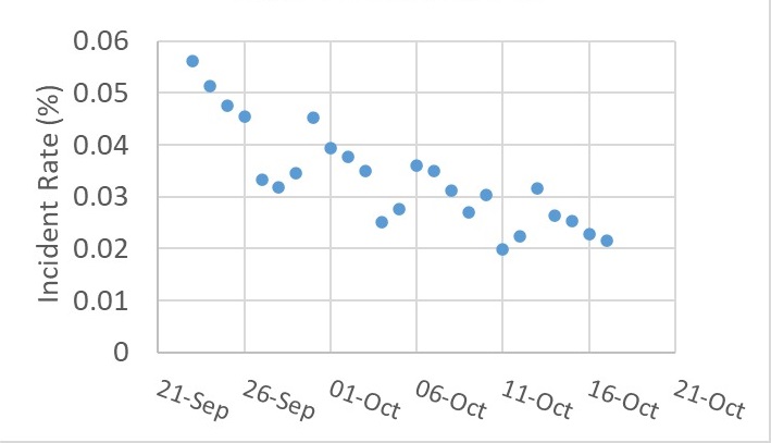
Puzzled by those periodic minima in the plot? It is an artefact in the data caused by the lower-than-usual number of tests on Sundays!

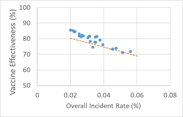
Yes, you guessed it right: the next step is to plot the incident rate with vaccine effectiveness. As expected, it is a straight line!

Correlation or Causation

It was still not easy to know what was happening. The whole observation can be a confounded outcome of something else. We have seen how chance plays its role in containing the disease outbreak (the post of swiss cheese!).

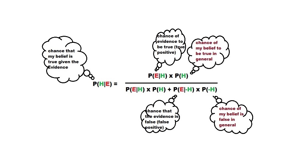
The next logical step is to perform the calculations and check if the trends are making sense. The calculations are:

Let P be the prevalence of the disease (incidence rate multiplied by some number to cover the who can still infect others at a given time). V represents the holes in the vaccination barrier, U is the holes in the unvaccinated (probability = 1), M is the holes in the mask usage, and n is the number of exposures that a person encounters. Here, I’ve stopped at mask as the only external factor, but you can add more barriers such as safe distance.

The chance of getting infected in n encounters with the virus = (1 – chance of being lucky in n encounters)
The chance of getting lucky in n encounters is = nCn x (chance of being lucky once)n x (chance of being unlucky once)0 = (chance of being lucky once)n.

The probability of being lucky once = (1 – chance of getting infected in a single encounter). The chance of getting infected is the joint probability of breaking through multiple barriers. So luck = (1 – P x M x V) for a vaccinated person and (1 – P x M) for an unvaccinated person. Note that V is related to 1 – prior assumed efficacy of the vaccine.

Finally, the effectiveness of vaccine = { [1 – (1 – P M )n] – [1 – (1 – P M V)n] } / {1 – (1 – P M)n}

You can already see from the expression that the vaccine effectiveness is a function of P, the prevalence. Repeat the calculations for a few incidence rates, and the results are plotted along with the actual data. The dotted line represents the estimation.

Key Takeaways

An apple to apple comparison between vaccines requires, among other things, the prevalence of the disease during the period of the efficacy trials. Part of the reason why many of the Covid 19 vaccines are showing modest efficacy levels lies in the extraordinary high incident rate of the illness prevailing through the last year and a half. A high prevalence of disease in society means a person, even though vaccinated, would encounter the virus several times, increasing the probability to get infected. Every such event is an additional test to the efficacy.

Vaccine Effectiveness and Incident Rates Read More »

The risk from the New Variant

As calamities from another variant of Covid19 is looming large, the omicron, be prepared for more confusing news in the coming days. It is also the right time to introduce the word risk. Risk has a specific technical meaning. It is the product of the likelihood of something to happen and the consequence.

Risk = likelihood x consequence.

Compare the delta variant with ones that came earlier. From the data, anecdotal evidence by individuals and evolutionary arguments, it became the public narrative that the consequence of infection with delta was similar to, or even mildly less dangerous. Did it mean the same for the risk? We can’t say until we know the likelihood. Delta turned out to be more than double as contagious as earlier ones. So the overall risk was much more than the first.

The second common argument was the case fatality rate. The CFR, as it is commonly known, was not high, they argued, but forgetting that almost a third of humanity was going to get it. A small fraction of a large number is still sizeable.

Black Swan Event

An extreme example of risk is the black swan event – a concept introduced by Nassim Nicholas Taleb through his book that carried the same name. These are unpredictable events and has infinite consequences.

Was the Covid pandemic a black swan event? As per the author himself, it was not a black swan event. People had predicted viruses attacks like these, and there were, however hypothetical, opportunities to control the disease at its onset, had there been a few steps taken by the originating country – be it intervention at the start or by just being more transparent.

But September 11 was one of them. It was never anticipated, and the consequence was enormous and far-reaching.

Delta variant

Black Swan Theory

Covid19 and Black Swan

The risk from the New Variant Read More »

Eating Natural and Other Lies

Most of the food you eat today is genetically modified, if not all! By genetic modification, I do not mean that the cultivar had gone through countless Petri dishes and a bunch of scientists injected solutions that would consciously and systematically modify specific parts of its DNA. Much milder than that, through a process called plant breeding, a fundamental process in agriculture.

Let me go a step further: humans cannot (or would not) make the transition from the Hunter-Gatherer society to the Agrarian without violating the rules of natural selection. We have seen Natural Selection before, and I want to repeat: Nature does not select anything. Nature only offers its playground and let the living species play random games. Some survive the game; we only get to see the survivors.

Humble Story of Staple Grains

Take wheat, rice and corn, which satisfy more than 50% of the calory requirements of the world. They all had their beginnings as grasses that bore too small seeds to attract any animals. Wild wheat seeds grew at the top of a stalk that spontaneously shattered and spread as far as possible, away from public sight, and quietly germinated. For that reason, they escaped early humans until a single-gene mutation caused a few plants to lose the capacity to shatter. For the wheat plant, this would be detrimental for the seeds cant fly to places and germinate. By the way, if I made you think that the plant was doing all these out of intelligence, let me rephrase – plants with such a defect won’t survive for long because of their limited capacity to spread their offspring.

However, such useless mutants were a lottery for humans as they got control of the entire growth and regrowth of the plants without losing any seeds. Wheat is now in her orchard. Occasionally, the already ‘unnatural’ plant gets another mutation, yielding larger seeds. From the plant’s viewpoint, what happened is a sheer wastage of its nutrients; after all, a seed, irrespective of its size, gets a single chance to become the next plant. Humans, on the other hand, love it and select only those bigger ones and grow.

For centuries we did this process without knowing what we were doing. Now we know the details, so much so that we know what parts of its genetic make-up need to change. And we also know how to change it!

Guns, Germs, and Steel by Jared Diamond

Eating Natural and Other Lies Read More »

Down Syndrome Continued

How odds and percentages can sometimes hide the big picture away from our eyes was the topic of an earlier post on Down Syndrome. Today, we continue from where we left off.

The data we analysed were livebirth from 10 states in the united states. That approach has a few issues. First, it included only 10 out of the 50 states. Second, and perhaps more importantly, the data covered only live births. In other words, there could be a survivorship bias to the data. What if children born with Down syndrome from different age-group-mothers have different chances of survival? Can it turn our analyses and insights upside down? Well, we don’t know, but we will find out.

Updated Data Including Stillbirths

Last time we sampled 10 states, 5600 live births and a total of 4.4 million mothers. Here we widen our net to cover 29 states, 12,946 births (live births and stillbirths) and a population of 9.8 million mothers. The messages are:

Women above 40 risk about 12 times higher than those younger than 35 to have babies with Down Syndrome. Yet, 54% of the mothers were 35 years or younger.

Not Done Yet

Is this all before we claim a logically consistent analysis? The answer is an emphatic NO. We still miss a major confounding factor that can potentially lead to a survivorship bias. It is the increased use of prenatal testing and termination of pregnancy for women older than 35. What we see at the end could be biased statistics of the probability distribution. So, the work is not done yet, and we will do more research in another post.

Selected Birth Defects Data from Population-Based Birth Defects Surveillance Programs in the United States, 2006 to 2010

Epidemiology Visualized: The Prosecutor’s Fallacy

Down Syndrome Continued Read More »

More On Prosecutors fallacy

Imagine a crime scene where the investigators were able to collect bloodstain. The sample was old, the DNA degraded, and the analysts estimated a relative frequency of 1 in 1000 in the population. Police found a suspect and got a DNA match. What is the chance that the suspect is guilty?

The prosecutor argues that since the relative frequency of the DNA match is 1 in 1000, the chance for the person to be innocent is 1 in 1000 and deserves maximum punishment. Well, the prosecutor made a wrong argument here. Imagine the city has 100,000 people in it. The test results suggest that there are about 100 people whose DNA can match the sample. So, the suspect is one of 100, and the chance of innocence only based on the DNA test is 99%.

Not Convinced? Let us use Bayes’ theorem.

P(INN|DNA) = P(DNA|INN)*P(INN)/ [P(DNA|INN)P(INN) + P(DNA|CRI)*P(CRI)]

P(INN|DNA) – the chance that the suspect is innocent given the DNA matches
P(DNA|INN) – chance of DNA match if the suspect is innocent = 1/1000
P(CRI) – prior probability that the suspect did the crime = 1 /100,000 (like any other citizen)
P(INN) – prior probability that the suspect is innocent = (1 – 1 /100,000)
P(DNA|CRI) – chance of DNA match given the suspect did the crime = 1 (100%)

P(INN|DNA) = (1/1000)* (1 – 1 /100,000) / ((1/1000)* (1 – 1 /100,000) + 1*(1/100000)) = 0.99

Does this mean that the suspect is innocent? Not either. The results only mean that the investigators must collect more evidence to file charges against the suspect.

More On Prosecutors fallacy Read More »

Swiss Cheese against Covid

The COVID-19 pandemic presented us with a live demonstration of science at work, much to the surprise of many who are not regular followers of its history. It gave a ringside view of the current state of the art, yet it created confusion among people whenever they missed consistency in the messaging, theories, or guidelines. The guidance on protective barriers—using masks, safe distancing, and hand washing—was one of them.

Swiss Cheese Model of Safety

The Swiss cheese model provides a picture of how the layered approach of risk management works against hazards. Let us use the model to check the underlying math behind general health advice on COVID-19 protection. I describe it through a simplified probability model.

The probability of someone getting infected by Covid 19 is a joint probability of several independent events. They are the probabilities:

  • an infected person who can transmit the virus in the vicinity (I)
  • to get inside a certain distance (D)
  • to pass through a mask (M)
  • to pass through the protection due to vaccination (V)
  • to get the infection after washing hands (H)
  • to infect the person once the virus is inside the body (S)

Infected person in the vicinity (I): is equal to the prevalence of the disease (assuming homogeneous mixing of people). Let’s make a simple estimate. These days, the UK reports about 50,000 cases per day in a population of 62 million. It is equivalent to an incident rate of 0.000806. Assume that an infected person can transmit the virus for ten days, and half of them manage to isolate themselves without passing the virus to others. The prevalence (proportion of people who can transmit the disease at a given moment) is 5 x 0.000806 = 0.0004032. Multiply by a factor of 2 to include the asymptomatic and the symptomatic but untested folks too into the mix. Prevalence becomes = 0.0008064 (8 in 1000).

To get inside a certain distance (D): If the person managed to stay outside the 2 m radius from an infected person, there could be zero probability of getting infected, but it is not practically possible to follow every time. Therefore, we assume she managed to stay away 50% of the time, which means a probability of 0.5 to get infected.

To pass through a mask (M): General purpose masks never offer 100% protection against viruses. So, assume 0.5 or 50% protection.

To pass through the protection from vaccination (V): The published data suggest that vaccination could prevent up to 80% of symptomatic infections. That means the chance of getting infected is 0.2 for the vaccinated.

The last two items – hand washing (H) and susceptibility to getting infected (S) – are assumed to play no role in protecting COVID-19. Infection via touching surfaces plays a minor role in transmission, and the latest variants (e.g. Delta) are so virulent that almost all get it once it is inside the body.

Scenario 1: Fully Protected Getting Infected Outdoor

Assume a person makes one visit outside in a day. The probability of getting the infection is = I x D x M x V x H x S = 0.008 x 0.5 x 0.5 x 0.2 x 1 x 1 = 0.0004 or the chance of not getting is 0.9996.

The person makes one visit for 30 days (or two visits for 15 days!). Her probability of getting infected on one of those days is = 1 – the probability she survived for 30 days. To estimate the survival probability, you need to use the binomial theorem. Which is 30C30 x 0.999630 x 0.0040 = 0.988. The chance of a fully protected person getting infected in a month outdoors is 1 – 0.988 or 12 in 1000!

Scenario 2: Fully Protected Person Indoor

The distance rule doesn’t work anymore, as the suspected droplets (or aerosols or whatever) are available everywhere. The probability of getting the infection is = I x D x M x V = 0.008 x 1 x 0.5 x 0.2 = 0.0008. This means the chance of not getting is 0.9992. 30-day chance is 1 – 0.976 = 0.024 or 24 in thousand.

Scenario3: Indoor Unprotected but Vaccinated

I x I x D x M x V = 0.008 x 1 x 1 x 0.2 = 0.0016. The chance of getting infected in a month = 1 – 0.95 or 5 in hundred.

Scenario4: Indoor Unprotected

I x D x M x V = 0.008 x 1 x 1 x 1 = 0.008. The chance of getting infected in a month = 1 – 0.78 or about 2 in 10 chance.

A bunch of simplifications were made in these calculations. One of them is the complete independence of items, which may not always hold. Some of these can be associated – a person who cares to make a safe distance may be more likely to wear a mask and get vaccinated. Inverse associations are also possible – a vaccinated person may start getting into crowds more often and stop following other safety practices. 

Second is the simplification of one outing and one encounter with an ill person. In reality, you may come across more than one infected. In the case of indoor, the suspended droplets containing the virus act as encounters with multiple individuals.

The case of health workers is different as the chances of encountering an infected person in a clinic or a medical facility differ from that in the general public. If one in ten people who come to a COVID clinic is infected, the chances of the health worker getting infected in a month are 95% if she wears an ordinary mask and comes across 100 patients daily. If she uses a better face cover that offers ten times more protection, the chance becomes about 25% in a month, or one in 4 gets infected even after getting vaccinated.

Bottomline

Despite all these barriers, people will still get infected. Small portions of large numbers are still sizeable numbers but do not get distracted by them. Use every single protection that is available to you. Those include vaccination, mask use, maintaining distance, and reducing non-essential outdoor trips. They all help to reduce the overall rate of infection.

Swiss Cheese against Covid Read More »

Prosecutors fallacy

We have seen that Bayes’ theorem is a fundamental tool to validate our beliefs about an event after seeing a piece of evidence. Importantly, it utilises existing statistics or prior knowledge to get to a conclusion. In other words, our hypothesis gets better representativeness by using Bayes’ theorem.

Take some examples. What are the chances that I have a specific disease, given that the test is positive? How good are my perceptions of a person’s job or abilities just by observing a set of personality traits? What are the chances that the accused is guilty, given that a piece of evidence is against her?

Validating hypotheses based on the available evidence is fundamental to investigations but is way harder than they appear, partly because of the illusion of the mind that confuses the required conditional probability with the opposite. In other words, what we wanted to find is a validation of the hypothesis given the evidence, but what we see around us is the chance of evidence if the hypothesis is true, because often, the latter is part of common knowledge.

To remind you of the mathematical form of Bayes’ theorem

Note that the denominator on the right-hand side is the probability of the evidence P(E)

Confusion between P(H|E) and P(E|H)

What about this? It is common knowledge that a running nose happens if you have a cold. Once that pattern is wired to our mind, the next time when you get a running nose, you assume that you got a cold. If the common cold is rare in your location, as per Bayes’ theorem, the assumption that you made require some serious validation.

Life is OK as long as our fallacies stop at such innocuous examples. But what if that happens from a judge, hearing the murder case? It is the classic prosecutor’s fallacy in which the size of the uncertainty of a test against the suspect is mistaken as the probability of that person’s innocence.

chances of crime, given the evidence = chance of evidence, given crime x (chance of crime/chance of evidence). Think about it, we will go through the details in another post. 

Prosecutors fallacy Read More »

Down Syndrome and Mistakes of Reasoning

We have debunked the mystery of covid infection among the vaccinated population in one of the earlier posts. Today we will see something similar but perhaps far easier to understand.

It is well-known that the risk of Down Syndrome increases with maternal age. For example, women above 40 risk about 11 times higher than those younger than 35 to have babies with Down Syndrome.

Yet, 52% of the mothers who give birth to children with Down Syndrome are 35 years or younger? Based on the data collected from 10 US states and the department of defence between 2006-2010, of the total number of 5600 live births, mothers of 2935 children were women younger than 35.

How did that happen? The simple answer is there were more mothers younger than 35! In the same population set, a whopping 3.7 million out of a total of 4.4 million were mothers below 35!

Small Fractions of Large Numbers

When the number of individuals in the less-risky category becomes very large, the absolute numbers of events also go up, despite its small relative chances to occur. For the vaccination case, the more the percentage of people get vaccinated, the more the absolute number of infected people from the vaccinated category if the society has a high prevalence of infection, which, in turn, is driven by the unvaccinated! But that is temporary – more people getting into the vaccination pool eventually steers the incidence rates down, slowly but steadily.

Selected Birth Defects Data from Population-Based Birth Defects Surveillance Programs in the United States, 2006 to 2010

Epidemiology Visualized: The Prosecutor’s Fallacy

Down Syndrome and Mistakes of Reasoning Read More »

The Big Short and The Assumption of Independence

In the last post, we have seen how banks make money by lending. To get estimates of profits and probabilities, we have assumed two conditions – independence and randomness. This time we look at cases where both these assumptions don’t hold.

Our bank is now making about 1.8 million annual returns with 2000 customers, who have been handpicked for their high credit scores and predictability to repay.

Want for More

An idea was proposed to the management to expand the firm and to increase the customer base. The argument was that even though adding more customers can reduce the predictability of defaulting, the risks could be managed by raising the interest rate a bit higher. Assurance was given that even for an assumed default rate of 5%, which is double the existing, by increasing the interest rate to 6.3%, the bank can make up about 8 million with 99% confidence. She has rationalised her calculations based on the law of large numbers, that the bank is unlikely to miss the target.

The expected value of profit = [interest rate x profit per loan x (1-default rate) – cost per foreclosure x default rate] x total number of loans.

For 20,000 loans, this will mean

[0.063 x 9000 x (1-0.05) – 100,000 x (0.05)] x 20,000

an earning of about 8 millions!

She further shows a plot of the simulation to support her arguments.

It convinced the management, and the company is now on an aggressive lending campaign. The firm has now 20,000 customers and makes a lot of money. A few months later comes a global financial crisis, and the firm is now bankrupt.

Assumption of Independence

To understand what happened to the bank, we should challenge the assumptions used in the original statistical calculations, especially the independence of variables – that one person defaults does not depend on the other. When there are many borrowers with varying capacities to repay, such crises prove detrimental to the business.

Assume a 50:50 chance, up or down, for everyone to default by a tiny fraction + / – 0.01 (1%) or between 0.04 and 0.06. Note that the average risk of default is still 5% but are no longer independent. Subsequently, the overall chances for making a loss has moved from 1% to 31%, but the average return is still around 8 million. A plot of the distribution of profits is below.

The plot is far from a uniform distribution as the central limit theorem would have predicted using an assumption of complete independence of variables.

The Big Short and The Assumption of Independence Read More »

Interest Rates and How not to Lose Money

In the previous post, we have seen how banks can lose money when they do the business of making money by disbursing loans. This time we will see how banks manage that risk by setting an interest rate for every loan they give. It means every lender needs to pay a fixed proportion of the borrowed money to the bank as a fee.

How does a bank set an internet rate? It is a balance between two opposing forces. If the rate is too low, it will not adequately cover the risk of defaults, and if it is too high, it could keep the customers away from taking loans.

Take the case of 10,000 banks each lends 90,000 dollars per customer to 2000 customers. Let’s say the bank sets an interest rate of 3% on the loans. After running Monte Carlo simulations, we can see the following.
The bank can earn a net profit of about 0.26 mln, but there is a 35% that it will lose money. In other words, 3500 banks won’t make money. The plot below describes this scenario.

Increase the interest rate to 3.8%. The expected profit is 1.6 mln, and there is about 1% of losing money. That sounds reasonable for a person to run the business. See below for the distribution.


Increase the interest rate to 5% and the profit if we manage to have all the customers intact is 3.77 mln and almost 0% chance of losing money. But a higher interest rate can drive customers away from this bank. Suppose three fourth of the customers have gone to other banks. The profit from 500 customers is less than a million and also there about 0.8% of losing money. Note that fluctuations increase to our estimations – net profits and the chances of making money – as the numbers are smaller (the opposite of the law of large numbers).

Interest Rates and How not to Lose Money Read More »