December 2021

Covid Stories 3 – The Gold Standard

December 31, 2021

Testing programs are not about machines but the people behind them.

We get into the calculations straight away. The equations that we made last time are:

$\text{Chance of Disease after a +ve result} = \frac{Sensitivity * Prevalence}{Sensitivity * Prevalence + (1-Specificity)*(1- Prevalence)} \\ \\ \text{Chance of No Disease after a -ve result} = \frac{Specificity* (1 - Prevalence)}{Specificity* (1-Prevalence) + (1-Sensitivity)*Prevalence} \\ \\ \text{Chance of Disease after a -ve result} = \frac{(1- Sensitivity )* Prevalence}{(1- Sensitivity )* Prevalence + Specificity*(1 - Prevalence)}$

Before we go further, let me show the output of 8 scenarios obtained by varying sensitivity and prevalence.

Case #	Sensitivity	Specificity	Prevalence	Chance of Disease for +ve (%)	Missed in 10000 tests
1	0.65	0.98	0.001	3	4
2	0.75	0.98	0.001	3.6	2.5
3	0.85	0.98	0.001	4	1.5
4	0.95	0.98	0.001	4.5	0.5
5	0.65	0.98	0.01	24	36
6	0.75	0.98	0.01	27	25
7	0.85	0.98	0.01	30	15
8	0.95	0.98	0.01	32	5

^{Chance of Disease for +ve = probability that a person is infected given her test result is positive. Missed in 10000 tests = the number of infected people showing negative results in every 10,000 tests.}

Note that I fixed specificity in those calculations. The leading test methods of Covid19, RT-PCR and rapid Antigen are both known to have exceptionally low false-positive rates or specificities of close to 100%.

Now the results.

Before the Spread

It is when the prevalence of the disease was at 0.001 or 0.1%. While it is pretty disheartening to know that 95% of the people who tested positive and isolated did not have the disease, you can argue that it was a small sacrifice one did for society! The scenarios of low prevalence also seem to offer a comparative advantage for carrying out random tests using more expensive higher sensitivity tests. Those are also occasions of extensive quarantine rules for the incoming crowd.

After the Spread

Once the disease has displayed its monstrous feat in the community, the focus must change from prevention to mitigation. The priority of the public health system shifts to providing quality care to the infected people, and the removal of highly infectious people comes next. Devoting more efforts to testing a large population using time-consuming and expensive methods is no more practical for medical staff, who are now required at the patient care. And by now, even the highest accurate test throws more infected people into the population than the least sensitive method when the infection rate was a tenth.

Working Smart

A community spread also rings the time to switch the mode of operation. The problem is massive, and the resources are limited. An ideal situation to intervene and innovate. But first, we need to understand the root cause of the varied sensitivity and estimate the risk of leaving out the false negative.

Reason for Low Sensitivity

The sensitivity of Covid tests is spread all over the place – from 40% to 100%. It is true for RT-PCR, even truer for rapid (antigen) tests. The reasons for an ultimate false-negative test may lie with a lower viral load of the infected person, the improper sample (swab) collection, the poor quality of the kit used, inadequate extraction of the sample at the laboratory, a substandard detector of the instrument, or all of them. You can add them up, but in the end, what matters is the concentration of viral particles in the detection chamber.

Both techniques require a minimum concentration of viral particles in the test solution. Imagine a sample that contains lower than the critical concentration. RT PCR manages this shortfall by amplifying the material in the lab, cycle by cycle, each doubling the count. That defines the cycle threshold (CT) as the number of amplification cycles required for the fluorescent signal to cross the detection threshold.

Suppose the solution requires a million particles per ml of the solution (that appears in front of the fluorescent detector), and you get there by running the cycle 21 times. You get a signal, you confirm positive and report CT = 21. If the concentration at that moment was just 100, you don’t get a response, and you continue the amplification step until you reach CT = 35 (100 x 2^{(35 – 21)} – 2 to the power 14 – is > 1 million). The machine suddenly detects, and you report a positive at CT = 35. However, this process can’t go forever; depending on the protocols, the CT has a cut-off of 35 to 40.

On the other hand, Antigen tests detect the presence of viral protein, and it has no means to amplify the quantity. After all, it is a quick point of care test. A direct comparison with the PCR family does not make much sense, as the two techniques work on different principles. But reports suggest sensitivities of > 90% for antigen tests for CT = 28 and lower. You can spare a thought at the irony that an Antigen test is sensitive to detect the presence of the virus that the PCR machine would have taken 28 rounds of amplification. But that is not the point. If you have the facility to amplify, why not use it.

The Risk of Leaving out the Infected

It is a subject of immense debate. Some scientists argue that the objectives of the testing program should be to detect and isolate the infectious and not every infected. While this makes sense in principle, there is a vital flaw in the argument. There is an underlying assumption that the person with too few counts to detect is always on the right side of the infection timeline – in the post-infectious phase. In reality, the person who got the negative test in a rapid screening can also be in the incubation period and becomes infectious in a few days. They point to the shape of the infection curve, which is skewed to the right, or fewer days to incubate to sizeable viral quantity and more time on the right. Another suggestion is to test more frequently so that the person who missed due to a lower count comes back for the test a day or two later and then caught.

How to Increase Sensitivity

There are a bunch of activities the system can do. The first in the list is to tighten the quality control or prevent all the loss mechanisms from the time of sampling till detection. That is training and procedures. The second is to change the strategy from analytical regime to clinical – from random screening to targetted testing. For example, if the qualified medical professional identifies patients with flu-like symptoms, the probability of catching a high-concentrated sample increases. Once that sample goes to the testing device for the antigen, you either find the suspect (covid) or not (flu), but it was not due to any lack of virus from the swab. If the health practitioner still suspects, she may recommend an RT PCR, but no more a random decision.

In Summary

We are in the middle of a pandemic. The old ways of prevention are no more practical. Covid diagnostics started as a clinical challenge, but somewhere along the journey, that shifted more to analytics. While test-kit manufacturers, laboratories, data scientists and the public are all valuable players to maximise the output, the lead must go back to trained medical professionals. A triage system, based on experiences to identify symptoms and suggested follow up actions, is a strategy worth the effort to stop this deluge of cases.

Covid Stories 2 – Predictive Values

December 30, 2021

We have seen the definitions. We will see their applications in diagnosis. As we have seen, both Sensitivity and Specificity are probabilities, and the diagnostic process’s job is to bring certainty to the presence of a disease from the data. And the tool we use is Bayes’ theorem. So let’s get started.

We tailor the Bayes’ theorem for our screening test. First, the chance of being infected after the person was diagnosed with a positive test. Epidemiologists call it positive predictive value or, in our language, the posterior probability.

Positive Predictive Value (PPV)

$P(Inf|+) = \frac{P(+|Inf) P(Inf) }{P(+|Inf) P(Inf) + P(+|NoInf) P(NoInf)}$

Looking at the equation carefully, we can see the following.
P(+|Inf) is the true positive or the sensitivity, and P(+|NoInf) is the false positive or (1 – Specificity). It leaves two unknown variables – P(Inf) and P(NoInf). P(Inf) is the prevalence of the disease in the community, and P(NoInf) is 1 – P(Inf).

$\text{Updated Chance of Disease} = \frac{Sensitivity * Prevalence}{Sensitivity * Prevalence + (1-Specificity)*(1- Prevalence)}$

And we’re done! Let’s apply the equation for a person who tested COVID-19 positive as part of a random sampling campaign in a city with a population of 100,000 and 100 ill people. The word random is a valuable description to remember; you will see the reason in a future post. Assume a sensitivity of 85% (yes, for your RT-PCR!) and a specificity of 98%.

Chance of Infection = 0.85 x 0.001 /(0.85 x 0.001 + 0.02 x 0.999) = 0.04. The instrument was of good quality, the health worker was skilled, and the system was honest (three deadly assumptions to make), yet she had only a 4% chance of infection.

Negative Predictive Value (NPV)

Now, quickly jump to the opposite: what is the chance someone who got tested negative, escapes the diagnostic web of the community?

$P(NoInf|-) = \frac{P(-|NoInf) P(NoInf) }{P(-|NoInf) P(NoInf) + P(-|Inf) P(Inf)} \\ \\ \text{Updated Chance of No Disease} = \frac{Specificity* (1 - Prevalence)}{Specificity* (1-Prevalence) + (1-Sensitivity)*Prevalence} \\ \\ = \frac{0.98 * 0.999}{0.98 * 0.999 + 0.15 * 0.001} = 0.9998$

There is a 99.98% certainty of no illness or a 0.02% chance of accidentally escaping the realm of the health protocol.

What These Mean

In the first example (PPV), a 4% chance of infection means relief to the person eventually, but there is a pain to do the mandatory ‘insolation’ as the system treats her as an infected.

The second one (NPV) is the opposite; for the individual, 0.02% is low; therefore, a test with medium sensitivity is quite acceptable. For the system, which wants to trace and isolate every single infected person, this means, that for every 10,000 people sampled randomly, there is a chance to send out two infected individuals into the society.

We have made a set of assumptions regarding sensitivity, specificity and prevalence. And the output is related to those. We will discuss the reasons behind these assumptions, the cost-risk-value tradeoffs, and the tricks to manage traps of diagnostics. But next time. Ciao.

Bayes’ rule in diagnosis: PubMed

False Negative Tests: Interactive graph NEJM

Covid Stories 2 – Predictive Values Read More »

Covid Stories 1 – Know the Jargons

December 29, 2021

Screening tests such as PCR are typically employed to test the likelihood of microbial pathogens in the body. Test results are estimates of probability and are evaluated by trained medical professionals to confirm the illness or to recommend any follow-up actions. Two terms that we have extensively used in the last two years have been the sensitivity and specificity of covid tests.

Sensitivity: Positive Among Infected, P(+|Inf)

Sensitivity is a conditional probability. It is not the ability of the machine to pick ill people from the population, although it could be related. But it is:

A test’s ability to correctly identify from a group of people who are infected.
P(+|Inf) – the probability of getting a positive result given the person was infected.

$\text{Sensitivity} = \frac{\text{Number of true positives (TP)}}{\text {Number of true positives (TP) + Number of false negatives (FN)}}$

A test has a sensitivity of 0.8 (80%) if it can correctly identify 80% of people who have the disease. However, it wrongly assigns 20% with negative results.

Specificity: Negative Among Healthy, P(-|NoInf)

A test’s ability to correctly identify from a group of people who are not infected.
P(-|NoInf) – the probability of getting a negative result given the person was not infected.

$\text{Specificity } = \frac{\text{Number of true negatives (TN)}}{\text {Number of true negatives (TN) + Number of false positives (FP)}}$

A test with 90% specificity correctly identifies 90% of the healthy and wrongly gives out positive results to the rest 10%.

Final Remarks

We’ll stop here but will continue in another post.
Sensitivity = P(+|Inf) = 1 – P(-|Inf). If you are infected, a test can either give a positive or a negative result (mutually exclusive probabilities). In other words, you are either true positive or false negative.

Specificity = P(-|NoInf) = 1 – P(+|NoInf). If you are healthy, a test can either give a negative or a positive test result – a true negative or a false positive.

Does a positive result from the screening test prove the person is infected? No, you need to know the prevalence to proceed further. We’ll see why we developed these equations and how we could use them to evaluate test results correctly.

Sensitivity and Specificity: BMJ

Covid Stories 1 – Know the Jargons Read More »

Bayesian Inference – Episode 2

December 28, 2021

Poisson, Gamma and the Objective

Last time we set the objective: i.e. to find the posterior distribution of the expected value, from a Poisson distributed set of variables using a Gamma distribution of the mean as the prior information.

Caution: Math Ahead!

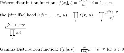
$\text{Poisson distribution function}: f(x_i|\mu) = \frac{\mu^{x_i}e^{-\mu}}{x_i!}; i = 1, ..., n. \\ \\ \text{the joint likelihood is} f(x_1, ..., x_n|\mu) = \displaystyle \prod_i f(x_i|\mu) = \displaystyle \prod_i \frac{\mu^{x_i}e^{-\mu}}{x_i!} \\ \\ = \frac{\mu^{\sum_i x_i}e^{-n\mu}}{\displaystyle \prod_i x_i!} \\ \\ \text{Gamma Distribution function}: f(\mu|a,b) = \frac{b^a}{\Gamma(a)}\mu^{a-1}e^{-b\mu} \text{ for } \mu > 0$

So we have a function and a prior. We will obtain the posterior using Bayes’ theorem.

$f(\mu|x_1, ..., x_n, a, b) = \frac{f(x_1, ..., x_n|\mu)f(\mu|a,b)}{\int_0^{\infty}f(x_1, ..., x_n|\mu)f(\mu|a,b) d\mu} = \frac{\frac{b^a}{\Gamma(a)} \frac{1}{ \displaystyle \prod_ix_i!} \mu^{a + \sum_i x_i - 1} e^{-(b+n)\mu}} {\frac{b^a}{\Gamma(a)} \frac{1}{ \displaystyle \prod_ix_i!} \int_0^{\infty}\mu^{a + \sum_i x_i - 1} e^{-(b+n)\mu} d\mu} \\ \\ = \frac{ \mu^{a + \sum_i x_i - 1} e^{-(b+n)\mu}} {\int_0^{\infty} \mu^{a + \sum_i x_i - 1} e^{-(b+n)\mu} d\mu} }$

The integral in the denominator will be a constant. Therefore,

$f(\mu|x_1, ..., x_n, a, b) \propto \mu^{a + \sum_i x_i - 1} e^{-(b+n)\mu}$

Look at the above equation carefully. Don’t you see the resemblance with a Gamma p.d.f, sans the constant?

$f(\mu|x_1, ..., x_n, a, b) \sim Gamma (a + \sum_i x_i , b+n)$

End Game

So if you know a prior gamma, you can get a posterior gamma based on the above equations. Recall the table from the previous post. The Sum of xi is 42000 and n is 7. Assume Gamma(6000,1) as a prior. This leads to a posterior of Gamma( 48000,8). Mean = 48000/8 and variance = 48000/8². The standard error becomes the square root of variance divided by the square root of n.

$\sqrt{\frac{4800/8^2}{7}} = 10.35 \text{confidence interval}, 4800/8 \pm 10.35 = (6010.35, 5989.65)$

Expanding the Prior Landscape

Naturally, you may be wondering why I chose a prior that has a mean of 6000, or where I got that distribution from etc. And these are valid arguments. The prior was arbitrarily chosen to perform the calculations. In reality, you can get it from several sources – from similar shops in the town, scenarios created for worst (or best) case situations and so on. Rule number one in the scientific process is to challenge, and two is to experiment. So, we run a few cases and see what happens.

Imagine you come up with a prior of Gamma(8000,2). What does this mean? A distribution with a mean of 4000 and a variance of 2000 (standard deviation 44). [Recall mean = a/b; variance = a/b² ]. The original distribution (Poisson) remains the same because it is your data.

Take another, Gamma(8000,1). A distribution with a mean of 8000 and a variance of 8000 (standard deviation 89).

Yes, the updated distributions do change positions, but they still hang around the original (from own data) probability density created by the Poisson function.

You may have noticed the power of Bayesian inference. The prior information can change expectations on the future yet retain the core elements.

Bayesian Inference – Episode 2 Read More »

Bayesian Statistics using Poisson Gamma

December 27, 2021

Do you remember the shopping mall example? The one which attracts about 6000 customers a day? Now your task is to establish an expected value, the number of customers in a given day, and a confidence interval around it. You have the customer visits from the previous week as a reference.

Day	Number of Visitors
Monday	6023
Tuesday	6001
Wednesday	5971
Thursday	6045
Friday	5970
Saturday	5950
Sunday	6040

The simplest way is: find out the mean, assume a distribution, and calculate the standard error. Let’s do that first. Since the number of visitors is counts, and we think their arrivals are random and independent (are they?), we choose to use Poisson distribution. Average of all those numbers give 6000, so it is

$x_i | \mu = Pois(\mu)$

In English, it meant: for fetching the distribution of counts at a given average (mu), we decided to use a Poisson distribution with a parameter mu.

The advantage of using the Poisson is that we can now get the variance easily. For Poisson, the mean and variance are both the same, equal to mu = 6000. Therefore,

$\text{standard error} = \frac{\text{standard deviation}} {\sqrt n} = \frac{{\sqrt{variance}}}{{\sqrt n}} \\ = \sqrt{\frac{variance}{n}} = \sqrt{(6000/7)} = 29 \\ \\ \text{95 p. c. confidence interval} = 6000 \pm 1.96 \text{ x } 29 = (6029, 5971)$

Bayesian Statistics

By now, you may have sensed that the best way to capture the uncertainties of customer visits is to consider the average too as a variable. After all, the present mean (6000) is just from a week’s data. Since the average is no more limited to integers but can also be fractions, we go for continuous distributions such as Gamma distribution to represent. In other words, a distribution of mu is my prior knowledge of average. And our objective is to get the updated mu or the posterior. So we are finally at the Baysian space for distributions or Bayesian statistics.

In Summary

You use the prior knowledge of the expected value (or average) through a Gamma distribution and apply it to the variable defined by a Poisson distribution. No marks for guessing: the posterior will be a Gamma! We will complete the exercise in the next post.

Bayesian Statistics using Poisson Gamma Read More »

The Gamma Distribution

December 26, 2021

Yet another type of distribution – the Gamma distribution. It is an example of a continuous distribution. i.e. the data (or the random variable) can take any values within its range. Look at a variable like the weight of people. The values it can take vary, from its lower to upper bound, through infinite micrograms in between. Whereas the distributions we have seen so far (binomial and Poisson) had to restrict themselves to counts or tries of integer values.

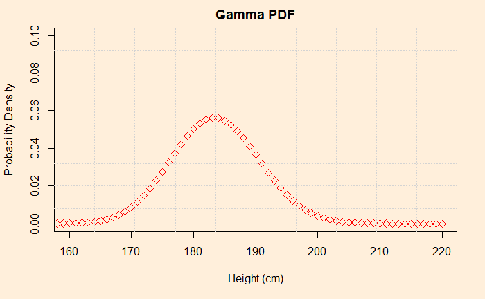
As we did earlier for Poisson and Binomial, we plot the actual distribution of the random variable, probability density function and cumulative distribution function. Take a set of fictitious data from 200 Dutch adults for their heights.

The R function that creates random variables is rgamma, and takes two parameters, a and b – rgamma(a,b). One interesting thing about these two parameters is that the expectation (mean) of the distribution is (a/b), and the variance is (a/b²). Similarly, dgamma gives the PDF of the distribution.

plot(dgamma(220, 670.15, 3.65), xlim = c(160,220), ylim = c(0,.1), xlab="Height (cm)", ylab="Probability Density", col = "red", cex = 1, pch = 5, type = "p", bg=23, main="Gamma PDF")
grid(nx = 10, ny = 9)

Gamma distribution is used for modelling systems that lead to positive outcomes. The distribution is not symmetric. For the example we created, the mean comes out to be 670.15/3.65 = 183.6 and standard deviation = square root (670.15/3.65²) = 7.1

There is a reason why I have introduced Gamma distribution immediately after the Poisson. That is for another post!

Height of Dutch Children from 1955 to 2009: Nature

The Gamma Distribution Read More »

The Count of Siméon Poisson

December 25, 2021

Take the example of this shopping mall that attracts about 6000 customers daily, between 10 AM and 8 PM. The shop manager wants to know the probability of 50 customers visiting the shop between 12:00 and 12:05 next Monday. How do you do it?

One way is to divide the time into several small intervals and do Bernaulli (binomial) trials at each interval using an average probability of someone arriving during that interval based on historical data. How do you divide the time – into hours, minutes or seconds? It seems a very laborious process.

Instead of dividing time into compartments and running Bernoulli trials for each of those intervals, what about taking the time-averaged visitors and estimating expected numbers for the given interval? This method of collecting timestamps instead of recording counts at regular intervals is the strength of the Poisson (/ˈpwɑːsɒn/)distribution. It is still a discrete distribution for the outcome still counts, but its time dimension is a continuum.

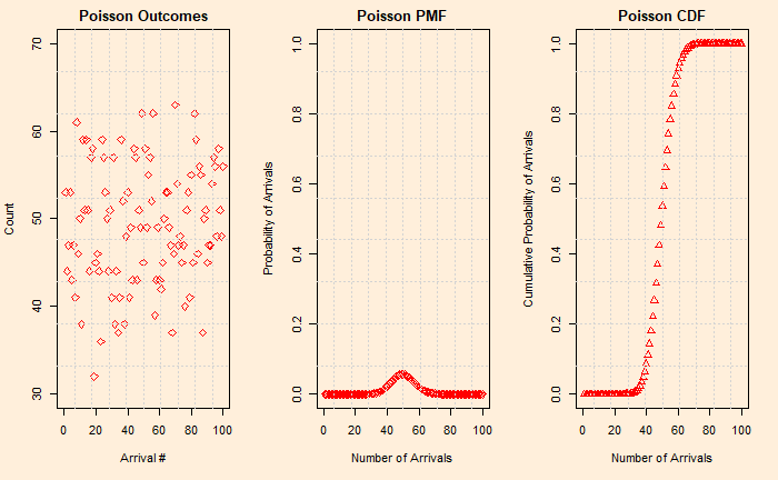
We do the same process that we did last time. Following are the event, PMF and CDF of the Poisson process.

The R code required to generate the above plots is below. Please take special note of the three special functions – rpois, dpois and ppois.

trial <- 100
xxx <- seq(1,trial)
lambda <- 10


par(bg = "antiquewhite1", mfrow = c(1,3))
plot(rpois(trial, lambda), xlim = c(0,100), ylim = c(0,25), xlab="Arrival #", ylab="Count", col = "red", cex = 1, pch = 5, type = "p", bg=23, main="Poisson Outcomes")
grid(nx = 10, ny = 9)

plot(dpois(xxx, lambda), xlim = c(0,20), ylim = c(0,1), xlab="Number of Arrivals", ylab="Probability of Arrivals", col = "red", cex = 1, pch = 5, type = "p", bg=23, main="Poisson PMF")
grid(nx = 10, ny = 9)

plot(ppois(xxx,lambda, lower.tail=TRUE), xlim = c(0,20), ylim = c(0,1), xlab="Number of Arrivals", ylab="Cumulative Probability of Arrivals", col = "red", cex = 1, pch = 2, type = "p", bg=23, main="Poisson CDF")

grid(nx = 10, ny = 9)

Now to answer the manager’s question.
The shop receives 6000 customers daily, i.e. an average of 50 customers every 5 minutes. It implies a Poisson function with an expected value (lambda) of 50. So what is the chance of 50 people arriving in a 5 min interval on a future day? It is dpois(50, lambda) = 5.5%

The Count of Siméon Poisson Read More »

Vaccine Kinetics – What Chemist Sees

December 24, 2021

Let me start with a disclaimer: this is purely for demonstration purposes. The numbers used in the following analysis should not be viewed as an accurate description of the complex biological processes in the body.

In an earlier post explaining vaccination, I had mentioned the law of mass action. It is also called chemical kinetics. For a chemist, everything is a reaction, and solving kinetic equations are the way of understanding the world around her.

Equations of life

Molecules react to form products. Consider the following hypothetical reactions.

(1) $\begin{equation*} \begin{aligned} V\xrightarrow{\text{k1}}2V \\ \end{aligned} \end{equation*}$

(2) $\begin{equation*} \begin{aligned} P\xrightarrow{\text{k2}}A \\ \end{aligned} \end{equation*}$

(3) $\begin{equation*} \begin{aligned} V + C \xrightarrow{\text{k3}} cell death \\ \end{aligned} \end{equation*}$

(4) $\begin{equation*} \begin{aligned} A + V\xrightarrow{\text{k4}} precipitate \end{aligned} \end{equation*}$

^{V represents virus, A for antibody, C for cells and P for blood plasma.}

As per the law of mass action, the speed of a reaction is related to its rate constant and concentrations of ingredients. The four items above translate to a set of differential equations,

(5) $\begin{equation*} \begin{aligned} \frac{dC_V} {dt} = 2 k1 C_V - k3 C_V C_C - k4 C_A C_V \\ \end{aligned} \end{equation*}$

(6) $\begin{equation*} \begin{aligned} \frac{dC_A} {dt} = k2 - k4 C_A C_V \\ \end{aligned} \end{equation*}$

(7) $\begin{equation*} \begin{aligned} \frac{dC_C} {dt} = - k3 C_V C_C \\ \end{aligned} \end{equation*}$

What do these equations mean?

All three equations have a rate (speed) term on the left and a set of additions (production) and subtractions (consumption) on the right.
The speed of each reaction is related to the concentrations of the constituents.
If a reaction rate constant increases, the speed of the reaction increases.
The production rate of antibodies (from blood plasma) is assumed constant.

Let us solve these three differential equations simultaneously. I used the R package ‘deSolve’ to carry out that job.

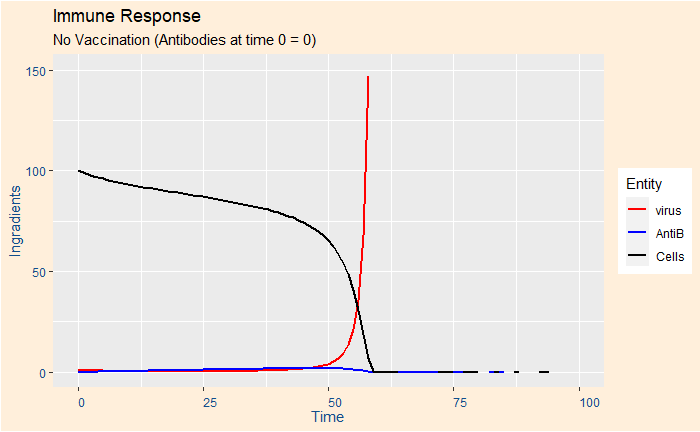
Case 1: A person in a risky group and no vaccination

Used the following set of (arbitrary) numbers: k1 = 0.45, k2 = 0.05, k3 = 0.01, k4 = 0.01. Intial concentrations (time = 0) Ca = 0, Cc = 100, Cv = 1.

You can see that the person is in real danger as all her cells have been attacked by the virus that multiplied exponentially.

Case 2: A person with healthy antibody production and no vaccination

Now, use exactly the same input, but the antibody production rate constant k2 is 4 x: k1 = 0.45, k2 = 0.2, k3 = 0.01, k4 = 0.01.

The initial growth of the virus was curbed down pretty fast by the antibodies and the person survived.

Case 3: Risky group and vaccination

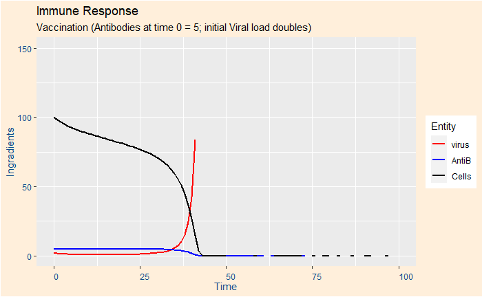
The parameters are the same as in case 1, but 5 units of antibodies are available at time zero (from vaccination).

Case 4: Risky group, vaccination, double viral load

Same as case 3, but the initial viral concentration doubled – from 1 to 2.

Case 5: Risky group, booster vaccination, double viral load

Same as case 4, but the antibodies from vaccination was double, or at ten units.

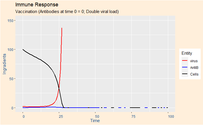
Case 6: No vaccination and double viral load

This case was created to show the speed at which the virus took control over the body. The parameters are exactly the same as case 1, but the initial virus load increased to 2 from 1.

In summary

These are simplistic ways of picturing what dynamics are going on in our body once a virus comes in. Treatments (mathematical) like these can also expand our imagination to newer ways of managing the illness. Say, can we find a way to reduce the rate constant k1 (viral replication)? Antiviral drugs such as ‘molnupiravir’ are expected to do precisely this.

Mechanism of molnupiravir-induced SARS-CoV-2 mutagenesis: Nature

Vaccine Kinetics – What Chemist Sees Read More »

Vaccine Effect – How the UK is Still Holding

December 23, 2021

The UK is one of the better-prepared countries, at the moment, to deal with Covid19. As per data published by the official website, 89.7% of the UK population, aged 12yr and above, have already taken at least one dose of vaccine, whereas 53% have taken three (data on 23/12).

It would be interesting to see how the country is doing so far against the virus. The following plot gives you various health-related parameters of Covid 19 infection. Critical parameters such as hospitalisations and deaths have been rescaled – both x and y axes – to coincide with the reported cases before the vaccine.

These are not perfect but are analyses capable of providing semi-qualitative insights. The peak rates in later 2020 – early 2021 suggest a case fatality ratio of about two (1 in 50) and a hospital admission case of 1 in 15. This was the situation before the vaccines became available. The ratios have come down significantly since then.

Corona Virus Data: the UK

Vaccine Effect – How the UK is Still Holding Read More »

Lebron and Free Throws

December 22, 2021

If Lebron has a 75% success rate from free throws, what is the chance that he makes nine or above out of 10 from the free throw line in the next game? We know how to solve this problem. Just apply the binomial relationship and estimate. Estimate the probability of nine and ten successes, and add them up. Like this:

₁₀C₉ x (0.75)⁹ x (0.25)¹ + ₁₀C₁₀ x (0.75)¹⁰ x (0.25)⁰ = 0.244

Three Games of Basketball

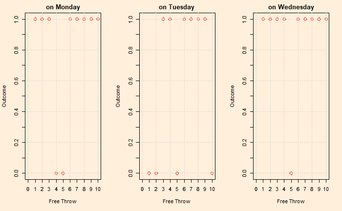
Obviously, you can not have 24.4% of doing something in a match – you either do it 100% or not do it at all. Let’s get into details of what these mean – using a few R functions and visualisations. Let’s look at three instances of Lebron throwing a total of ten, at the success rate of 0.75. Run the following R code:

trial <- 10
xxx <- seq(1,trial)
prob_x <- 0.75

game_play <- function(n){
  sample(c(0,1),size = 1, replace = TRUE,prob = c((1-prob_x), prob_x))
  }

xtick<-seq(0, trial, by= 1)
ytick<-seq(0, 1, by=0.1)


par(bg = "antiquewhite1", mfrow = c(1,3))
plot(xxx, sapply(xxx, game_play), xlim = c(0,trial), ylim = c(0,1), xlab="Free Throw", ylab="Outcome", col = "red", cex = 1, pch = 5, type = "p", bg=23, main="on Monday")
grid()
axis(side=1, at=xtick, labels = TRUE)
axis(side=2, at=ytick, labels = FALSE)

plot(xxx, sapply(xxx, game_play), xlim = c(0,trial), ylim = c(0,1), xlab="Free Throw", ylab="Outcome", col = "red", cex = 1, pch = 5, type = "p", bg=23, main="on Tuesday")
grid()
axis(side=1, at=xtick, labels = TRUE)
axis(side=2, at=ytick, labels = FALSE)

plot(xxx, sapply(xxx, game_play), xlim = c(0,trial), ylim = c(0,1), xlab="Free Throw", ylab="Outcome", col = "red", cex = 1, pch = 5, type = "p", bg=23, main="on Wednesday")
grid()
axis(side=1, at=xtick, labels = TRUE)
axis(side=2, at=ytick, labels = FALSE)

He made it on Wednesday; on Tuesday and Monday, he didn’t. We used an R function called sample, a random sample generator coupled with a probability condition of 0.75 for success. Each time you run this code, you get three plots with different outcomes.

PMF and CDF

You must have heard about Probability Mass Functions, Cumulative Density Functions etc. They are pretty handy to understand more about the winning chances in distributions, and we will use them to answer the original question.

Let’s place three plots side by side. The one on the left is what could happen in an actual game. The one on its right is a plot of chances for each try if you play the game several times, and the one on the extreme right is the plot of the cumulative probability distribution. You can get cumulative by adding the probabilities in the PMF one by one, from left to right.

Now let us answer the original question by looking at the plot. The one on the left is the least useful to make any conclusions. If you look at this one-off game, you may presume that Lebron would not make 9 or 10 in a game. It is the answer by someone who saw only one game or has scant regard for statistics!

Calculating from the PMF plot is simple: add the density at nine successful shots and ten successful shots together (I have marked 9 with a vertical line as a guide). And 0.188 + 0.056 = 0.244. Using the last plot (CDF), you calculate everything above 8. Or subtract from 1, the number corresponding to 8; you get 1 – 0.756 = 0.244.

Lebron and Free Throws Read More »

December 2021

Before the Spread

After the Spread

Working Smart

Reason for Low Sensitivity

The Risk of Leaving out the Infected

How to Increase Sensitivity

In Summary

Further Reading

Positive Predictive Value (PPV)

Negative Predictive Value (NPV)

What These Mean

Sensitivity: Positive Among Infected, P(+|Inf)

Specificity: Negative Among Healthy, P(-|NoInf)

Final Remarks

Poisson, Gamma and the Objective

Caution: Math Ahead!

End Game

Expanding the Prior Landscape

Bayesian Statistics

In Summary

Equations of life

What do these equations mean?

Case 1: A person in a risky group and no vaccination

Case 2: A person with healthy antibody production and no vaccination

Case 3: Risky group and vaccination

Case 4: Risky group, vaccination, double viral load

Case 5: Risky group, booster vaccination, double viral load

Case 6: No vaccination and double viral load

In summary

Three Games of Basketball

PMF and CDF