A sailor sails between two ports. At each port, he stays with a woman, both of whom want to have a child with him. The sailor is initially reluctant but changes his mind and tosses a coin to decide: if it’s a head, he will have a child with one and if it’s tail, with both. If heads come up, he will open up The Sailor’s Guide to Ports, and whichever port, out of the two, features earlier, he will choose the woman on that port.
If A is the son of the sailor, what is the probability that he is an only son?
Yesterday night (or earlier today, for some), the Miami Heat beat Boston Celtics to win the Eastern Conference final of the NBA, thus qualifying for the ultimate showdown against the Denver Nuggets. The Heat made it in the seventh game after both teams had tied at 3-3.
In many ways, the matchup has been a nightmare that threw sports analysts and Las Vegas for a complete spin. For those who missed the plot, Celtics were the pre-series favourites but lost the first three matches to the Heat. The Heat obtained the momentum to make the fourth win for a sweep but lost the next three games and gave the momentum back to the Celtics. And the Celtics, not knowing that they have this thing called momentum, lost cheaply against the Heat.
The momentum of sports
Momentum is a term borrowed from physics, defined as the product of mass and velocity, a parameter with magnitude and direction. Journalists use it to represent some internal force of nature (psychology) that moves entities (sports teams, stock prices) to one direction based on their immediate past performances.
Momentum, like a hot hand, positive energy and negative energy, is a type of cognitive illusion. An argument that is often used to explain a complex or a random process. While hot hands may be partially explainable as it happens due to someone’s mood or a form on a day, this momentum thing happens over a few days. The three-match stretch may appear to you like a sequence, but each game breaks for 45 hours before the next one; most professional teams recover from such setbacks. And every game becomes a new matchup, unconnected to the previous; like a coin toss.
One can argue it was a reverse momentum that happened in this series. The fourth match became the must-win for the Celtics. And as it happened several times in the past two years, they successfully dragged themselves out of the hole, not once, but three times. Then it became a must-win for the Heat (well, also for the Celtics), which they successfully executed.
Imagine you get a chance to buy a coffee shop. Here is what the owner tells you. The current sales = $ 74,000 /yr Shop rent = $30,000 /yr Employee salary = $25,000 /yr Coffee beans = $15,000 /yr The cost of furniture and coffee machine = $45,000
How much are you willing to pay?
Market value
A simple valuation shows the shop can generate $4,000 a year (74,000 – 30,000 – 25,000 – 15,000) after paying for the rent, salaries and the purchase of the coffee beans. If you feel the shop will generate the same forever, you can do a simple (perpetuity) formula of 4000 / 0.1 = 40,000; 0.1 represents the discount rate of 10%. So you are willing to pay a maximum of $40,000.
The owner reminds you that she spent 45,000 just a few weeks ago to renovate. Will you change your mind? Sadly, it shouldn’t. The cost the owner sunk in the past can’t change the value it generates in the future. The buyer politely replies that she could get $500 more ($4,500) every year if she invested that 45,000 in the market at a 10% return. So what the owner spent (the book value) is immaterial to the buyer who calculated the market value.
Movie or football
Mat bought a ticket for a movie by paying $25. Just before he starts, he gets a phone call from John, who invites him to watch a football match. Mat likes football and John’s company, yet declines the invite because he has already spent the ticket price of the movie.
The money Mat spent is sunk, and what matters now is what gives him a good time (movie vs football with friends). But Mat falls for the sunk cost fallacy, the bad feeling for the loss on things that have already been spent against a better return in the future.
The concord of failures
The fallacy of sunk cost is common in big projects. Companies often hesitate to shut down projects midway when even they realise that it’s getting expensive and the product won’t make any economic benefit. They rationalise they invested too much to quit.
Social scientists hypothesise three reasons for this fallacy
The loss aversion
Desire not to appear wasteful
To force one to do things that otherwise won’t happen
Psychology of decision making
The sunk cost fallacy is a powerful force that impacts decision-making. The issue with sunk costs is that they are the things of the past, but we pay too much attention to them. It’s the same feeling that keeps you attending the whole show of a terrible movie, eating everything ordered even when you are full, or continuing a nonfunctional relationship solely because the couple spent four years of their life together.
Reference
Sunk Costs: The Big Misconception About Most Investments: Sprouts
We have seen that the two most commonly used ways of summarising the centre of variation of observed values are the mean and the median. The mean is the numerical average, and the median is the mid-point.
Andrew Vickers uses the following example to illustrate the need for two parameters and the issue when there are outliers. Seven people with annual incomes of $85,000, $50,000, $60,000, $40,000, $75,000, $100,000 and $45,000 are in a dinner. Bill Gates walks in. What is the new distribution of the salary in the room?
Before Gates
Before Mr Gates walked in, the average salary was ($85,000 + $50,000 + $60,000 + $40,000 + $75,000 + $100,000 + $45,000) / 7 = $65,000. To estimate the median, we first need to arrange the numbers in ascending order, $40,000, $45,000, $50,000, $60,000, $75,000, $85,000, $100,000, locate the midpoint, i.e., $60,000, which is the median.
After Gates
The picture changes once Mr Gates enters the room. Let’s assume his annual income (!) is $ 1 B (the highest number I could envision). The mean is = 1,000,455,000 / 8 = $ 125 million and a bit. And the median? ($60,000 + $75,000)/2 = $67,500.
You might say the median ($67,500) better represents the crowd of upper-middle-class people (and one billionaire). The mean, the so-called average, appears helpless here.
The session cannot be complete without invoking my favourite plot of all – the box plot.
You may have noticed that 7 out of 8 fall below the mean.
Reference
What is a p-value anyway? 34 Stories to Help You Actually Understand Statistics: Andrew Vickers
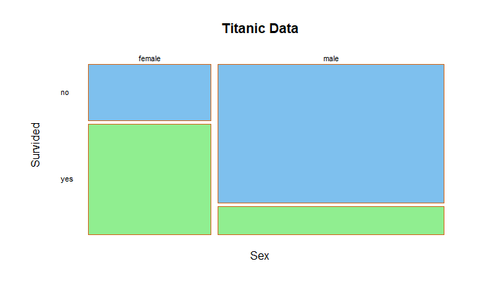
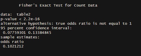
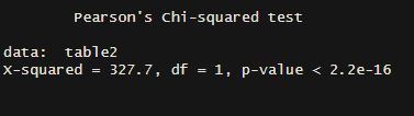
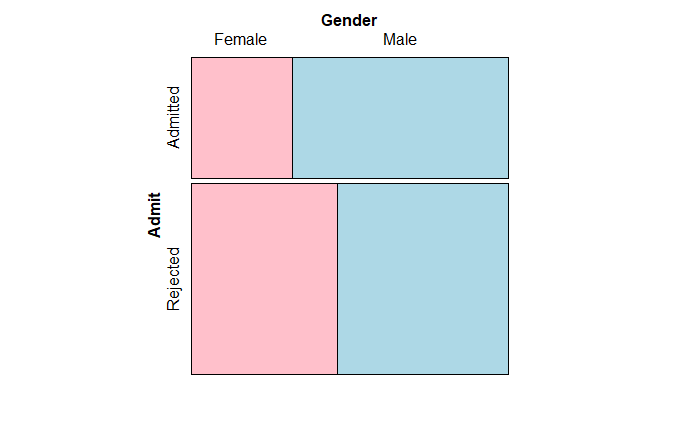
We have seen Berkeley data in the previous post and refreshed the concept of Simpson’s paradox. Here we introduce a handy visualisation of such data using mosaic plots.
The following R code generates the mosaic plot for the overall admission. The code requires the ‘vcd’ package.
mosaic( ~   Gender + Admit, data = berk_data,
       highlighting = "Gender", highlighting_fill = c("pink", "lightblue"),
       direction = c("v","h"))
The lower width of the pink panel on the admission (top) suggests a smaller number of females (89) compared to males (512). The smaller width of the top pink panel compared to the bottom pink panel indicates lower admission rates for females (proportional to the application rate). Smaller heights of pannels indicate more rejection than admission.
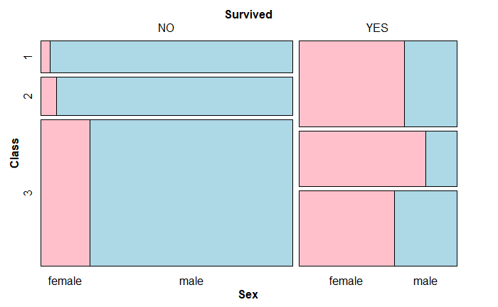
Once the data is stratified to include the department, the picture changes to the following.
mosaic( ~ Dept  + Gender + Admit, data  = berk_data,
       highlighting = "Gender", highlighting_fill = c("pink", "lightblue"),
       direction = c("v","v","h"))
Most of the pink panels on the top are more than or equal to the ones on the bottom, suggesting better admission rates for females. You can check the last table of the previous post and recognise that the admission rates of departments A and B are more than 50%, and the rest are lower. Lastly, the number of male applicants is much more in those two departments (width of the blue panel compared to pink).
We have seen Simpson’s paradox in one of the earlier posts. A famous one was the discrepancy in observed admission rates of men and women from six departments at Berkeley. Here is what the data shows; the dataset is available on GitHub.
Admit
Gender
Dept
Frequency
Admitted
Male
A
512
Rejected
Male
A
313
Admitted
Female
A
89
Rejected
Female
A
19
Admitted
Male
B
353
Rejected
Male
B
207
Admitted
Female
B
17
Rejected
Female
B
8
Admitted
Male
C
120
Rejected
Male
C
205
Admitted
Female
C
202
Rejected
Female
C
391
Admitted
Male
D
138
Rejected
Male
D
279
Admitted
Female
D
131
Rejected
Female
D
244
Admitted
Male
E
53
Rejected
Male
E
138
Admitted
Female
E
94
Rejected
Female
E
299
Admitted
Male
F
22
Rejected
Male
F
351
Admitted
Female
F
24
Rejected
Female
F
317
The paradox
If one considers the university as a whole, here is the summary
Admit
Gender
#
Admitted
Male
1198
Rejected
Male
1493
Admitted
Female
557
Rejected
Female
1278
Total
4526
Proportion of Male admitted = 1198 /(1198+1493) = 0.45
Proportion of female admitted = 557/(557 + 1278) = 0.30
There is a difference in success rates for men and women. But what about department-wise ‘discrimination’? Here are the success rates of males and females in each department.
Department
Male
Female
A
0.62
0.82
B
0.63
0.68
C
0.37
0.34
D
0.33
0.35
E
0.28
0.24
F
0.06
0.07
Success rates of females are at par or even higher in every department! Let’s probe further and check where they applied against the success rates.
Department
% Male Applied
% Female Applied
Admission Rate (%)
A
30
6
64
B
21
1
63
C
12
32
35
D
15
20
34
E
7
21
25
F
14
19
6
Total
100
100
Women preferred more competitive departments with lower acceptance rates, whereas more men opted for departments with better acceptance rates.
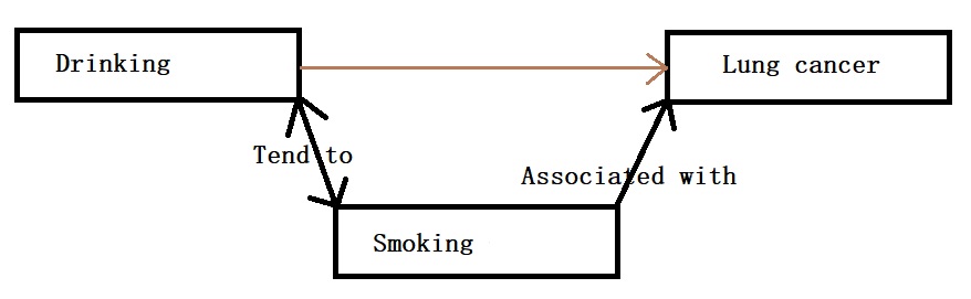
We have seen confounders before; it is a factor that associates with both exposure and outcome, thereby deceiving investigators of a causal relationship between the two.
For example, smoking is a confounder that misleads people to conclude that drinking can lead to lung cancer. In reality, smokers have a higher tendency to drink, and smokers have a higher tendency to get lung cancer. Until you stratify and find the impact of drinking on smokers and non-smokers, you are unlikely to figure out the error.
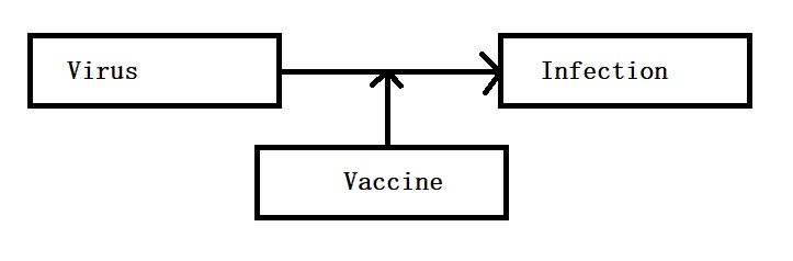
On the other hand, if the variable impact the outcome and not the exposure, it is an effect modification. A simple example is the immunisation status of an individual can impact the person’s susceptibility to getting the infection from the virus.