Maximum Likelihood Estimation
This is my 1000th post. While the likelihood of reaching post # 1000 in as many days is one topic for a future post, today we specifically develop some intuition around MLE or the maximum likelihood estimate.
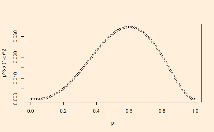
A coin lands H, H, T, T, H. How likely is this to happen? A simplistic way is to think that this coin always lands in this pattern (H, H, T, T, H). We know that is not credible. Let’s assign the coin a probability p (“the parameter”) to land heads. So, the question we want to answer is: at what probability (of occurrence for heads), p, does the likelihood maximise?
Step 1: What is the probability of observing the sequence HHTTH? Let’s assume all flips are independent. The probability is
p x p x (1-p) x (1-p) x p = p3 x (1-p)2
Step 2: What is the value of p at which the likelihood of observing HHTTH is maximised? We will take help from calculus, take a derivative, equate to zero, and solve for p.
3p2 x (1-p)2 – 2 p3 x (1-p) = 0
3(1-p) – 2p = 0
p = 3/5 = 0.6
Ok, the MLE for this sequence is 0.6. But what is the probability of the sequence happening? For that, substitute the value of p in the equation,
0.6 x 0.6 x (1-0.6) x (1-0.6) x 0.6 = 0.03456
Conclusion: if the coin lands on heads 60% of the time, the probability of seeing the sequence HHTTH is 3.456%. 3.456% may appear small, but it is better than any other p.
Continuous distribution
If a person’s height is 66 inches, which population is she from? It is unusually rare that a region has only people 66 inches tall. We assume that people’s heights follow a normal distribution with a standard deviation (say, 4). So, the question becomes: What is the most likely distribution that person is from?
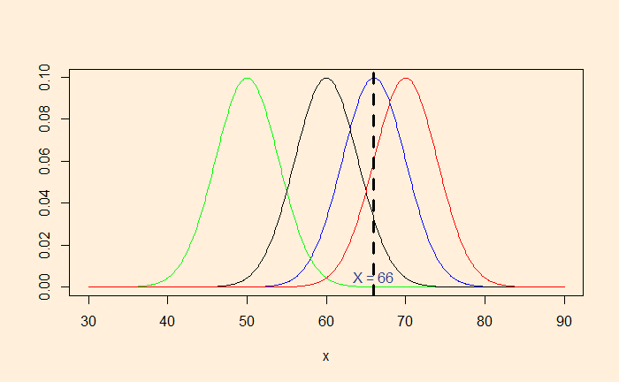
Here are a few distributions with the standard deviation 4. By placing a market at x = 66, you can observe that the distribution with mean = 66 is the most likely (the highest point) to represent the observed data.
Instead, we collected two data, 66 and 58 inches. The blue curve strongly supports 66, but not much 58. MLE will balance the probabilities so that it can include both the data.
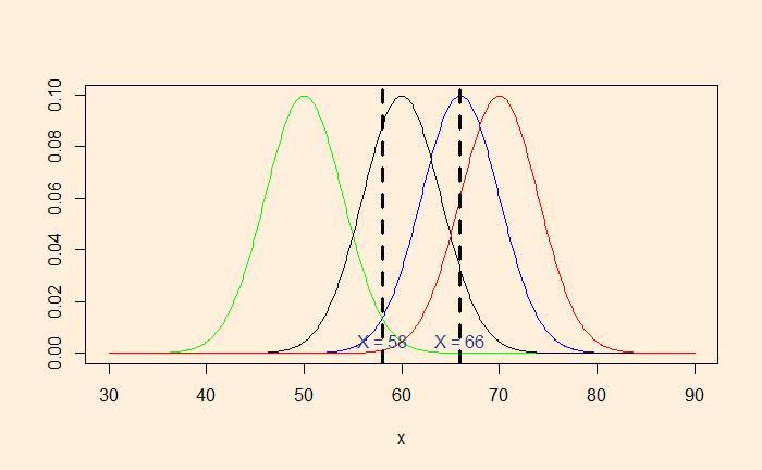
The average of 66 and 58 (= 62) will maximise the likelihood.
Reference
Maximum Likelihood Estimation: Brian Greco – Learn Statistics!
Maximum Likelihood Estimation Read More »