We will discuss a cognitive preference that can impact our decision-making. The mere-exposure effect, also known as the familiarity principle, is the human tendency to prefer what is familiar to us and to make us allergic to changes. As per the Encyclopedia of Social Psychology, it is “a phenomenon that simply encountering a stimulus repeatedly somehow makes one like it more”.
One direct application of this effect is in the area of advertisements. Marketing people have used this technique to perfection for brands and products through repeated campaigns to encourage customers towards them.
It’s been a while, so let’s do a probability problem. I found this one in the youtube channel “MindYourDecisions“. If it rains on a day, the probability of rain tomorrow increases by 10%; if not, it reduces by 10% for the next day. What is the probability that it will rain forever within a few days if the chance to rain today is 60%?
Let Px be the chance of raining forever, starting from a day x% rain. We can write the following equations. Note that P100 means it will rain today and every day from there. On the other hand, P0 suggest no rain today and, as a result, it continues.
P100
1
P90
0.9P100 + 0.1P80
P80
0.8P90 + 0.2P70
P70
0.7P80 + 0.3P60
P60
0.6P70 + 0.4P50
P50
0.5P60 + 0.5P40
P40
0.4P50 + 0.6P30
P30
0.3P40 + 0.7P20
P20
0.2P30 + 0.8P10
P10
0.1P20 + 0.9P0
P0
0
Substituting the end value (P0 = 0) for the term P10 and working upwards,
P100
1
P90
0.9P100 + 0.1P80
0.998P100
P80
0.8P90 + 0.2P70
0.98P90
P70
0.7P80 + 0.3P60
0.93P80
P60
0.6P70 + 0.4P50
0.82P70
P50
0.5P60 + 0.5P40
0.67P60
P40
0.4P50 + 0.6P30
0.51P50
P30
0.3P40 + 0.7P20
0.35P40
P20
0.2P30 + 0.8P10
0.22P30
P10
0.1P20 + 0.9P0
0.1P20
P0
0
The value of the last term, 0.998P100 can be evaluated by substituting P100 = 1. Repeating the exercise, now downwards,
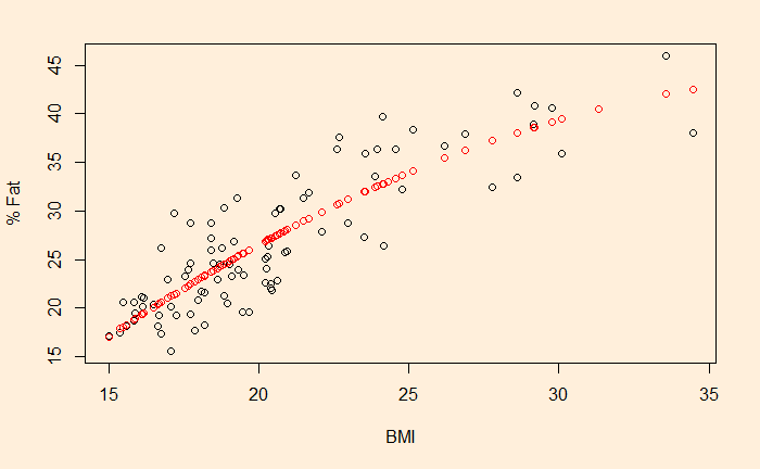
We have seen linear regression last time. While fitting a line could be a good start, one needs to exercise care before choosing it as the default. For example, see the plot below.
It gives the relationship between body mass index and body fat percentage, taken from Regression Analysis Book by Jim Frost. Warning: I’m not sure if the data was simulated or data.
Check what happens if you try and fit a straight line!
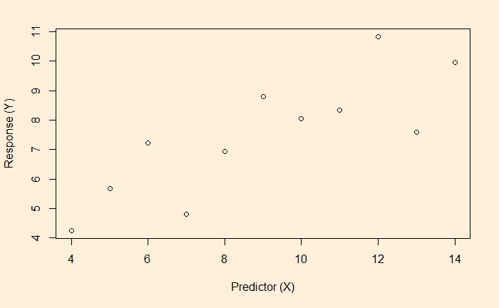
OLS is the short form for ordinary least squares and is a linear regression method. The process is also known as curve fitting informally. The objective is to find the relationship between the dependent (the y) and independent (the x) variables; one eventually gets (to predict) the variation of y from the variation of x. In case you forgot, here is the scatter plot of the data.
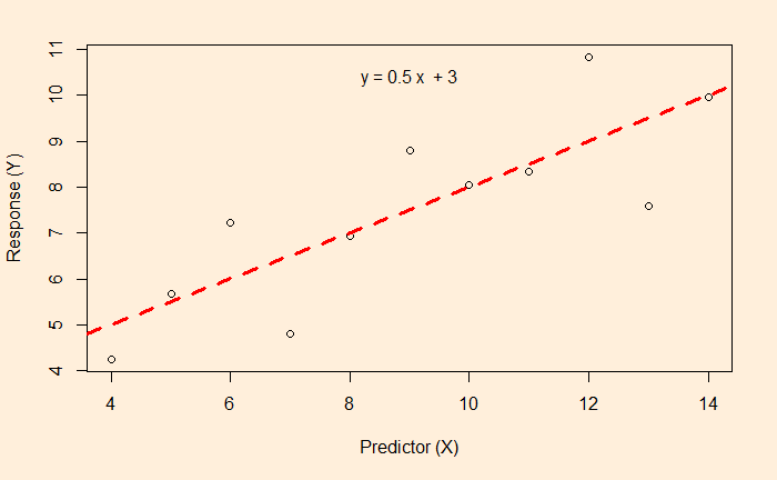
Outliers are data points that don’t fit the model well. Outliers are data points that don’t fit the model well. Let’s take the previous example we did earlier.
Here is an updated dataset with the addition of a new point corresponding to x = 13 but doesn’t make sense to the otherwise overall behaviour.
You can see that the outlying data has pulled the right side of the regression line up.
Let’s run another popular choice for CO2 removal – aforestation or planting trees. In this scenario,100% of the available land is used for afforestation.
Now, compare that with a highly reduced rate of deforestation.
The outcome is the same – a very marginal reduction of temperature rise.
It takes time for trees to grow
The key reason for the aforestation failure is the time it takes for the trees to grow. The time till 2100 is less than 80 years, and an 80-year-old tree is still young!
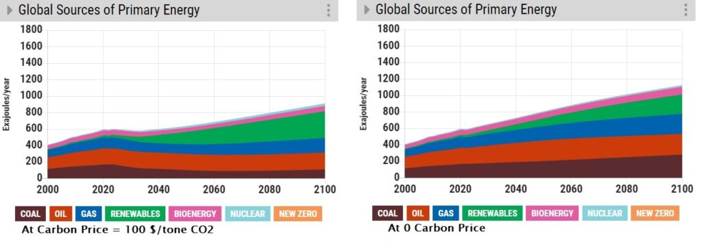
We saw last time in the En-ROADS simulation results the power of carbon price to make a difference in the decarbonisation pursuit. From the results, you can see what a carbon price of 200 $/tone of CO2 can do to the energy mix:
At that price, a whole set of renewable investment options is available to an investor. And only after such investment does the change happen. But that is not enough for someone to set billions of dollars in renewable projects. The magic word is uncertain. How could an investor trust the carbon price at a future date to be true? What happens if the governments backtrack from today’s commitments or remove schemes (say, cap and trade) altogether? So the political uncertainty for an investor is too high to depend on the carbon price.
CCFD – the hedge against uncertainty
One way to reduce the uncertainty and encourage investments in clean energy is a carbon contract for difference (CCFD). CCFD is the commitment by the government to pay out to companies a specified amount of money in case there is a difference between the expected and the actual.
We will use En-ROADS to simulate the impact of the carbon price on climate goals. First, we switch off the efficiency buttons from the previous runs. And set the carbon price to 100 $/tone CO2.
It would be interesting to see how the price impacted the energy mix.
As you can see, the market turned away from Coal in favour of more renewables. We now raise the price to 200 $/tone CO2.
We saw En-ROADS last time as a tool to simulate the impact of steps we can/should to en route to a decarbonised future. Now, we simulate scenarios, starting with energy efficiency.
The silver bullet?
There is a reason to start with this. A lot of people (policymakers) think energy efficiency offers huge opportunities in the journey of decarbonisation, and it comes at zero cost (or even at negative cost)! I suspect the famous McKinsey curve has something to do with this belief. I suspect the famous McKinsey curve has something to do with this belief. But let’s test the hypothesis.
Simulation results
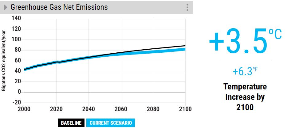
First, the baseline: we have seen before that if we maintain the status quo, we end up with a temperature rise of +3.6 oC compared to the pre-industrialised levels. We do run the model in two steps. First, we make set maximum efficiency changes (transport and building) at the current volume of electrification, i.e. no growth.
The underlying assumptions for this simulation are a growth rate of 5% per year from 2023 and a 5% rate for buildings and industries (new and retrofitted).
Now, switch on electrification to the mix. Here we added 100% electrification of new transport (rail and road) and buildings from 2023, which we know, can not be true!
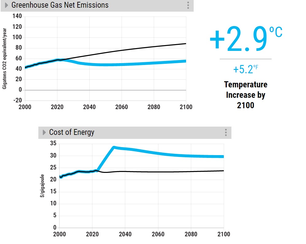
So, what are we seeing? Even at extremely optimistic rates of energy efficiency and electrification rates, we will miss the climate goal of 2100. Building electrification also causes an increase in energy costs in the medium term.
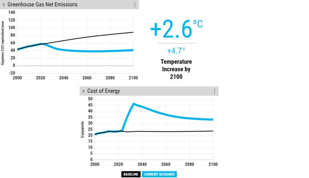
Ignoring building electrification still makes most of the results (+2.9 oC) at no cost. The question now is: here is an option (improving efficiency) that can still make a good stride towards decarbonised work at no cost, but not realised. From an economic standpoint, this doesn’t make sense – a market failure.
Limiting “global warming to well below 2, preferably to 1.5 oC, compared to pre-industrial levels”, is the main objective of the Paris agreement, which is a legally binding international treaty on climate change. However formidable the goal might appear, there are pathways to achieve it with the help of deploying appropriate technologies and policies.
We introduce En-ROADS, the online climate simulation tool developed by Climate Interactive, Ventana Systems, UML Climate Change Initiative, and MIT Sloan, to create the results from various scenarios. The simulator provides a set of outputs, such as the temperature increase by 2100, CO2 emissions, cost of energy, sea level rise, and about 100 others from a selection of inputs that include 1) energy efficiency and electrification, 2) growth, 3) land use, 4) carbon capture technologies, and 5) Carbon pricing and other policies.
The screenshot of the interface provided below shows how the interactive lets the user handle some serious physics and math of climate change as child’s play and free of charge!