Continuing from the previous post, we will apply the normal-normal Bayesian inference to the height problem. The general format of the Bayes’ rule is:
Since there are two parameters involved in the normal distribution, we have to have either a double integral in the denominator or choose one of the parameters, say the standard deviations, as known. So, we assume the standard deviation to be 4.0 in the present case. Let’s take the mean for the prior to be 69, the standard deviation to be 3 and see what happens. Therefore,
Now we have everything to complete the problem.
You can see a few things here: 1) the prior has moved a bit in the direction of the data but is still far from it, 2) the posterior is narrower than the prior.
We have seen how to come up with estimates of events based on assumed prior data using Bayesian inference. For discrete events that are rare, we have Poisson likelihood, and on such occasions, we use a Gamma prior and get a gamma posterior. In the same manner for Shaq, wefound that the best one for estimating his success (or the lack of it) of entering Whitehouse is a binomial distribution. Once a data point is collected (one attempt), you update the chances using a beta distribution as a prior, and you get beta as the posterior.
Here is a new challenge you have a task to estimate the male height distribution of a particular country. We know from the examples of other countries that normal distributions describe the height distributions. A normal distribution has two parameters – mean and standard deviation, and our challenge is to estimate these parameters for our new country. We start with a set of hypotheses, use the available data and apply Bayesian inference to reach the goal.
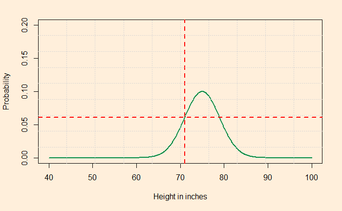
Assume that I have collected data from the region, and it is 71 inches. Now I assume that the means ranges from 50 to 80 inches and the standard deviation from 1 to 4. Collect five hypotheses (purely random) from them as follows:
Now ask the question: what is the likelihood that my distribution of the new country is N(75, 4) given that I have collected data of 71 inches? Same for the rest four of the hypotheses. It can be estimated utilising the standard tables or using the R function dnorm(71, 75,4) = 0.06049268. The Pictorial representation is below.
Before applying the Bayes’ theory, we should realise that 1) we need prior probabilities for each of the above five hypotheses and 2) we can have infinite hypotheses, not just five! Then we can apply the formula as we did before.
It is a conjugate problem (the prior will be a pdf), and the right prior is a normal distribution, making it a normal-normal problem. How to complete the exercise using normal-normal is something we will see next.
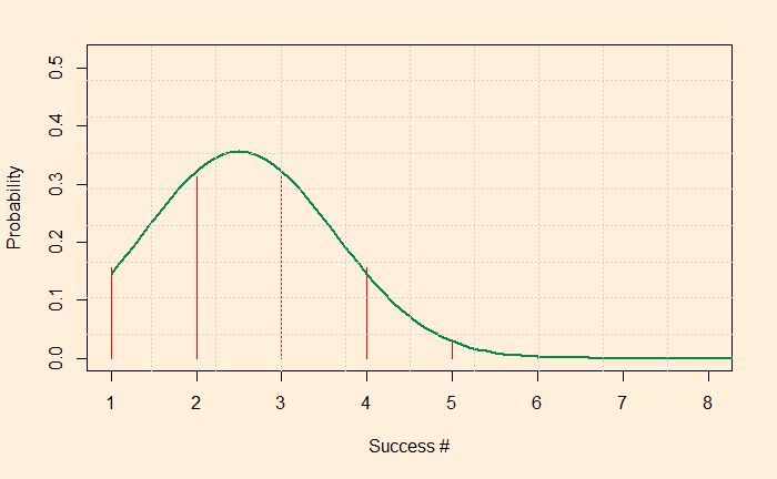
We have seen it before: what is the chance of getting three heads if you toss a coin five times? The answer is about 30%. You know how to do it: 5C3 (0.5)3(0.5)5-3 = 0.3125. The distribution representing the probability of each success when a coin is tossed five times is given by the PMF of binomial.
We have used the following R code (the dbinom function for PMF) to generate this plot.
xx <- seq(1,30,1)
p <- 0.5
q = 1 - p
toss <- 5

par(bg = "antiquewhite1")
plot(dbinom(xx,race,p), xlim = c(1,8), ylim = c(0,0.52), xlab="Success #", ylab="Probability", cex = 1, pch = 5, type = "h", main="", col = ifelse(xx >= 24,"#006600",'red'))
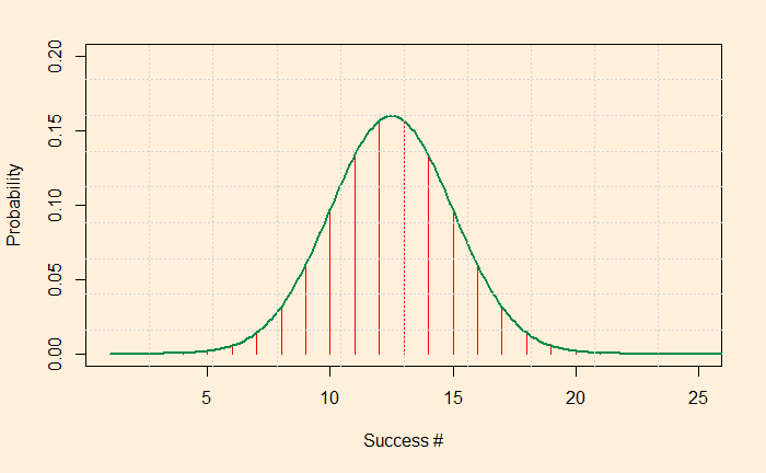
If you look at the distribution carefully, you will see that it resembles a normal distribution. For the normal distribution, we need a mean and a standard deviation. The mean is easy: you multiply the total number of tossing with the probability of success in one toss, i.e., 5 x 0.5 = 2.5. The variance of a binomial distribution is N x p x (1-p); the standard deviation is its square root. Let’s try making a normal distribution and superpose.
xx <- seq(1,30,1)
p <- 0.5
q = 1 - p
toss <- 5

par(bg = "antiquewhite1")
plot(dbinom(xx,toss,p), xlim = c(1,8), ylim = c(0,0.52), xlab="Success #", ylab="Probability", cex = 1, pch = 5, type = "h", main="", col = ifelse(xx >= 24,"#006600",'red'))

xx <- seq(1,30,0.1)
mean_i <- toss*p
sd_i <- sqrt(toss*p*q)

lines(xx, dnorm(xx, mean = mean_i , sd = sd_i ), xlim = c(0,30), ylim = c(0,0.2), xlab="Evidence for guilt", ylab="Frequency", col = "springgreen4", cex = 1, pch = 5, type = "l", bg=23, lwd = 2, main="")
grid(nx = 10, ny = 9)
Looks like the green line representing the normal distribution is almost passing through binomial values. We will soon see that when the number of trials (N) is large, the binomial becomes indistinguishable from a normal distribution. For N is 25. Like this:
This post is not a commentary on the book Selfish Gene by Richard Dawkins, although I do recommend the book. But this is around how to understand what is selfishness.
It seems scientists often forget about the common public when it comes to naming their books or concepts. That way, the title, selfish gene, is just another one: survival of the fittest, natural selection, god particle, the list goes on. None of these phrases represents what they truly meant. God particles have nothing to do with god, survival does not correlate with any physical fitness, or there is nobody in nature to select or reject anything.
Selfishness in biology simply means the ability to survive no matter what. It has little to do with a species’ deliberated actions using its brain, such as mating (or not mating), not sharing resources, stealing or killing. It only means making copies and preserving genes by passing from generation to generation.
What a headless virus can do
Take the case of the most popular show in town, the novel coronavirus, SARS-CoV-2 or Covid-19. The virus has two parts, the outer envelope, which has a bunch of proteins, including the famous spikes, all embedded in a lipid membrane and the inside material that contains the genome, a single-stranded RNA, preserved nicely on a protein called the nucleocapsid or N-protein. The genome is long and contains information to make new viruses using someone else’s workshop, the human cells.
The virus thus mobilises human cell machinery (e.g. ribosomes) to replicate. It creates billions of copies that infect millions of people. And the virus does all these without having a body or a brain!
Brain doesn’t need to follow
Human genes, too, want to preserve themselves. They are also selfish and want to be immortal. But it has a master, the human brain, which can overrule the instincts for the greater good. It may have inherent altruism, but more importantly, it is trainable based on a value system. While the brainless gene wants and will long for eternal life, you, as a human, can prefer not to have offspring. You may stop taking sugar, run for hours when no lion is chasing, donate organs to strangers.
Parkinson’s disease accompanies the loss of dopaminergic neurons responsible for synthesising the neurotransmitter dopamine. Dopamine is often known as the molecule that controls motivation through a reward mechanism. Naturally, the chemical earned the reputation of being responsible for addiction, pleasure etc.
An illness negatively correlated with an addiction-causing chemical is thus an ideal candidate for seeing confounding. Let’s take some well-known addictions, namely coffee, smoking and alcohol.
Coffees’ negative correlation with Parkinson’s is something we have seen earlier. Next up is smoking, and lo and behold, smoking is associated with a lower tendency of Parkinson’s disease! Now, I have no choice but to search for alcoholism. This one appears more complex. Most of the studies showed no association or weak negative correlation.
Confounding, is it?
It has all the ingredients to be a confounding phenomenon. But until a new study came up with a mechanistic explanation – Nicotins effect on neuron survival.
Estimation of risk is a very desirable quality to have because it can improve survival rates. Earlier, we have seen the definition of risk as the product of probability and impact. But for most people, it is something far more intuitive and personal. Risk perception, as they are called, may come from recent experiences, news headlines or simply from the lack of knowledge of something. One dominant example is the perception that people live more risky life today than in the past. Data suggest this is incorrect.
Incorrect estimation of risk comes from our mind’s inability to quantify probabilities. That is why when asked about the risk of an even, experts looks at the past (annual incident rate), whereas people consider the future (catastrophic potential). An example is how laypeople perceive the risk due to nuclear power (very high) versus what the experts’ estimate (one of the safest energy technologies)! Wikipedia reports about 30 incidents related to radiations in history, and the deaths were in single digits in 21 of them. Now compare that with a million annually due to coal!
Regression to mean misleads a lot of us. We have seen the concept of regression before. In simple language: most of our superlative achievements and miserable falls are statistical, although you may like to credit them to your superior skillset or discredit to utmost stupidity. With statistical, I did not mean sheer luck but something milder; more like, ‘perhaps unexpected, but not improbable‘.
In flight training, the experienced trainers think that praise after an incredibly smooth landing follows a poor landing, and harsh criticism after a poor landing leads to improvement. They believe in this because 1) it fits with some old-generation stereotypes, 2) that’s what they see (but how often?) or 3) memories of such instances persist longer.
Regression to mean suggests that an above-the-average data point has more chance to be succeeded by something lower-than-the-average. Well, is that not why something called an average exists? Look at this problem differently. What is the probability that a given performance is outstanding? It has to be less than one and likely closer to zero; else, the dictionary meaning of the word outstanding will require a new definition. Having one such incident occurred, what is the chance of one more such event (or even rarer) to occur? It will be a product of two fractions, and the resulting number will be even smaller.
What happened here is a failure to understand how probability and regression work. So next time, if Lebron’s son doesn’t become a first-round pick, don’t blame the chap. What happened to him was normal, whereas what occurred to his father was rare!
The outcome of the debate of nature versus nurture is a foregone conclusion. It confused people in the past, but we now know that the problem is an example of confounding. Vaci et al. have published a paper in 2019 in a longitudinal study tracking chess players throughout their careers. And the results showed the importance of numerical intelligence and deliberate practice to master and retain chess skills. Nonlinear interactions between the two suggest that intelligent people benefit more from practice.
The work looked at 90 chess players across their careers – the Elo rating and the number of tournament games played. Three levels of intelligence – verbal, figural and numerical – were followed but found that the numerical has the highest correlation to the performance.
The nonlinearity of behaviour means people of different ages climbed up the rating ladder differently. For 20-year olds, players with an IQ of 120 benefited more from the same amount of practice than ones with IQs of 100 at lower practice regimes. At that stage, more practice of both groups reduced the gap between their performances. At the very high levels of practice, the higher intelligent folks started deviating from others for better performance. The behaviour is represented in the schematic below.
The joint influence of intelligence and practice on skill development throughout the life span: PNAS
2015 was a landmark year for international policymaking. The year started with the United Nations Sustainable Development Goals (SDG) and ended with the climate goals, known as the Paris Agreement.
While 17 goals constitute the SDG, we focus on the first one i.e., No poverty in all its forms everywhere. Extreme poverty per the international poverty line (IPL) stands at USD 1.90/day. The World Bank presented two additional levels at USD 3.20/day and USD 5.50/day. It means getting people out of these should be the priority of the rest of us.
Contradicting goals
At first sight, you may find a contradiction between these two goals. It is well known that carbon dioxide emissions increase with wealth (consumption), and targetting SDG1 flags an inconvenient truth of raising it further.
Asymmetry in emissions
A paper published last week (14/Feb/2022) in Nature Sustainability addresses this problem. The work computes the potential CO2 emissions due to the upliftment of masses from absolute poverty and proves that the increase is negligible in comparison with the total. The reason lies in the asymmetry of emissions between the rich and the poor. Let’s understand the math behind the claims.
In 2017, 9.2% of the global population lived in extreme poverty of less than USD 1.90/day, and their average footprint is 0.4 tCO2 (per person per year). Another 14.9% live between 1.90 and 3.2 USD/day. They contribute around 0.6 tCO2. The last batch includes about 19.5% of people who live between 3.2 and 5.5 USD/day and at 0.9 tCO2/person/year. To put these numbers in perspective, see the following:
CO2 Footprint (tCO2/person/yr)
Global Average
4.5
US Average
14.5
top 10% US
54.9
Europe Average
6.3
Imagine we aim to lift the people in 1.90 (0.74 Billion) and 3.2 (1.2 Billion) USD/day bracket to 5.5 (1.6 Billion). It would mean 3.5 billion people in the USD 5.5 per day category with an average footprint of 0.9 tCO2. So the current emissions from the 3.5 billion = 0.74 * 0.4 + 1.2 * 0.6 + 1.6 * 0.9 = 2.46 GtCO2/yr. The new emissions (after 1.9 and 3.2 are raised above the 5.5 mark) = 0.74 * 0.9 + 1.2 * 0.9 + 1.6 * 0.9 = 3.19 GtCO2/yr. The difference = 3.19 – 2.46= 0.73 GtCO2/yr. The additional emissions, 0.73 is about 2% of the current global emission of 36 GtCO2/yr. And they live in India, China, Sub-Saharan Africa and South and Southeast Asia.
Here is an update on the global carbon dioxide (CO2) situation. If you need a background on the topic, you may go to my previous posts on this topic. The world needs to restrict the average temperature rise, from the pre-industrial level, to below 1.5 oC to avert catastrophic climate changes. For simplicity, take 1850 as the start of the counting. 1.5 oC corresponds to a median concentration of CO2 of about 507 ppm (parts per million) in the atmosphere (425-785 ppm at 95% confidence range).
From these numbers, one can estimate the quantity of CO2 we could throw into the atmosphere before it crosses the critical concentration. The maximum remaining quantity of CO2 is known as the Carbon Budget.
Now the numbers: Based on the latest estimate at the beginning of 2022,
Item
Quantity
Unit
Carbon Budget
420
GtCO2
CO2 Concentration
414.7
ppm
Global anthropogenic CO2 emissions (2021)
39.4
GtCO2
Global fossil CO2 emissions (2021)
36.4
GtCO2
Gt = Gigatonne = billion tonnes; anthropogenic = originating from human activity; 39.4-364. = 3GtCO2 comes from land usage
Spending Wisely
At the current rate, the budget will be over by 2032! There is a resolution from the global fraternity to reduce the net CO2 emission to zero by 2050. If we trust that commitment, one can draw spending scenarios to reach the target. If we spend the remaining 420 Gt in equal chunks, we can do it by spending 15 Gt every year until 2050 and put a hard brake, which is not practical, given the present lifestyle of 36.4 Gt/yr. Another scenario is by reducing 8% every year. Notice that an 8% yearly reduction corresponds to halving every nine years. In other words, the spending in 2030 has to be half of what we did last year.
And How are we doing?
Nothing to cheer about (so far). The emission figures from the last three years have been:
Year
Total CO2 Emitted (GtCO2)
at 8% reduction (GtCO2)
2019
36.7
36.7
2020
34.8
33.8
2021
36.4
31
Since we know the real reason for the decline in 2020, the global shutdown due to pandemic, the 8% reduction remains a project without any evidence of progress.