Using this equation, we get P(Defective) = P(Machine1)P(Defective|Machine1) + P(Machine2)P(Defective|Machine2) + P(Machine3)P(Defective|Machine3) = 0.5×0.05 + 0.25×0.1 + 0.25×0.12 = 0.08 or 8% chance.
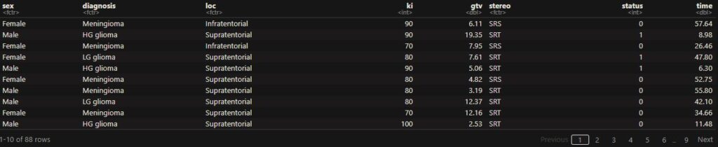
Here is a step-by-step process for performing a chi-squared test of independence using R. The following is a survey result from a random sample of 395 people. The survey asked about participants’ education levels. Based on the collected data, do you find any relationships? Consider a 5% significance level.
The chi-squared = 8.0061 at degrees of freedom = 3. As the p-value = 0.04589 < 0.05, we reject the null hypothesis; the education level depends on the gender at a 5% significance level.
A recent survey showed the number of children per household as follows:
# Children per household
Population
0
4.3
1
1.0
2
2.3
3
0.3
4
0.2
5
0
Check how the data compares with a Poisson distribution with lambda = 1.
You may recall that lambda is the expected value of Poisson distribution. First, we create the Poisson probabilities for each category from the number of children per household = 0.
We have seen family-wise error rate (FWER) as the probability of making at least one Type 1 error when conducting m hypothesis tests.
FWER = P(falsely reject at least one null hypothesis) = 1 – P(do not reject any null hypothesis) = 1 – P(∩j=1n {do not falsely reject H0,j})
If each of these tests is independent, the required probability equals (1 – α)n, and FWER = 1 – (1 – α)n
For example, if the significance level is 0.05 (α) for five tests, FWER = 1 – (1 – 0.05)5 And, if you make n = 100 independent tests, FWER = 1 – (1 – 0.05)100 = 0.994; guaranteed to make at least one Type I error.
One of the classical methods of managing the FWER is the Bonferroni correction. As per this, the corrected alpha is the original alpha divided by the number of tests, n. Bonferroni corrected α = original α / n
For five tests, FWER = 1 – (1 – 0.05/5)5 = 0.049; and for 100 tests FWER = 1 – (1 – 0.05/100)100 = 0.049
Imagine a fair coin is tossed 10 times to test the hypothesis, H0: the coin is unbiased. The coin likely lands on heads (or tails) in about 5 (or 4, 3, 2) of those. If it landed 4 times on heads and 6 in tails, we can do a simple chi-squared test to verify. chi-squared = (4 – 5)2 /5 + (4 – 5)2 /5 = 0.4. 0.4 is too low; we can’t reject null
But what happens if all the tosses land on tails? chi-squared = (0 – 5)2 /5 + (10 – 5)2 /5 = 10. We reject at 99% confidence level. We know the probability of this happening is (1/2)10 = 1/1024.
chisq.test(c(0,10),p=c(0.5,0.5))
	Chi-squared test for given probabilities

data:  c(0, 10)
X-squared = 10, df = 1, p-value = 0.001565
What about 1024 players, each having a (fair) coin toss 10 times each?
1 - dbinom(0, 1024, 1/1024)
0.63
In other words, there is a possibility that one person will reject the null hypothesis and conclude that the coin is based! An incorrect rejection of a null hypothesis or a false positive result. In other words, if we test a lot (a family) of hypotheses, there is a high probability of getting one very small p-value by chance.
Here are Kaplan – Meier plots for males and females taken from the results of a cancer study. The data comes from the ‘BrainCancer’ dataset from the R library ISLR2. It contains the survival times for patients with primary brain tumours undergoing treatment.
At first glance, it appears that females were doing better, up to about 50 months, until the two lines merged. The question is: is the difference (between the two survival plots) statistically significant?
You may think of using two-sample t-tests comparing the means of survival times. But the presence of censoring makes life difficult. So, we use the log-rank test.
The idea here is to test the null hypothesis, H0, that the expected value of the random variable X, E(X) = 0, and to build a test statistic of the following form,
X is the sum of the number of people who died at each time.
R does the job for you; use the library, survival.
The outcome variable in survival analysis is the time until an event occurs. Since studies are often time-bounded, some patients may survive the event at the end of the study, and others may stop responding to the survey midway through. In either case, those patients’ survival times are censored. As censored patients also provide valuable data, the analyst gets into a dilemma of whether to discard those candidates.
Let’s examine five patients in a study. The filled circles represent the completion of the event (e.g., death), and the open circles represent the censoring (either dropping out or surviving the study’s end date).
The survival function, S(t), is the probability that the true survival time (T) exceeds some fixed number t. S(t) = P(T > t) S(t) decreases with time (t) as the probability decreases as time passes.
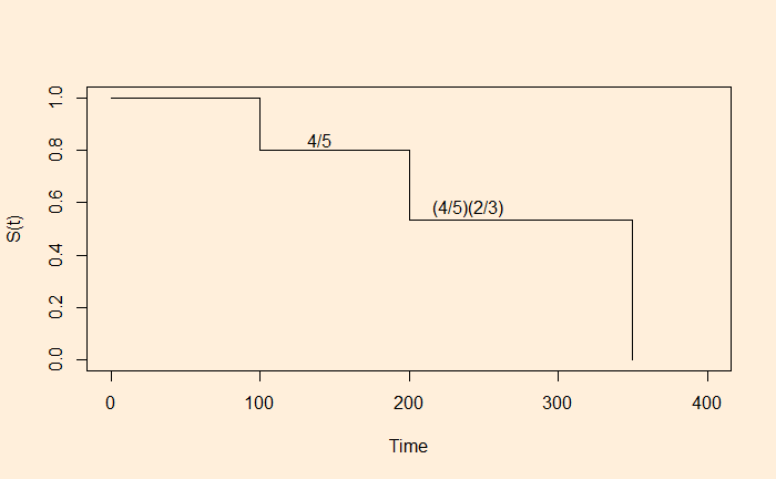
In the above example, how do you conclude the probability of surviving 300 days, S(300)? Will it be 1/3 = 0.33 (only the one survived out of three events, ignoring the censored) or 3/5 = 0.6 (assuming the censored candidates also survived)? What difference does it make to the conclusion that one of them dropped out early when she was too sick?
Kaplan and Meier came up with a smart solution to this. Note that they worked on this problem separately. Their survival curve is made the following way. 1) The first event happened at time 100. The probability of survival at t = 100 is 4/5, noting that four of the five patients were known to have survived that stage.
2) We now proceed to the next event, patient 3. Note that we skipped the censored time of patient 2.
Now, two out of three survived. The overall survival probability at t = 200 is (4/5) x (2/3).
3) Move to the last event (patient 5); the survival function is zero ((4/5) x (2/3) x 0). This leads to the Kaplan -Meier plot:
We have seen survival plots before. Survival plots represent ‘time to event’ in survival analysis. For example, in the case of cancer diagnostics, survival analysis measures the time it takes from exposure to the event, which is most likely death.
These analyses are done following a group of candidates (or patients) between two time periods, i.e., the start and end of the study. Candidates are enrolled at different times during the period, and the ‘time to event’ is noted down. Censoring is a term in survival analysis that denotes when the researcher does not know the exact time-to-event for an included observation.
Right censoring The term is used when you know the person is still surviving at the end of the study period. Let x be the time since enrollment, and then all we know is the time-to-event ti > x. Imagine a study that started in 2010 and ended in 2020, and a person who was enrolled in 2018 was still alive at the study’s culmination. So we know that xi > 2 years. The same category applies to patients who missed out on follow-ups.
Left censoring This happens in observational studies, where the risk happens before entering the studies. Because of this, the researcher cannot observe the time when the event occurred. Obviously, this can’t happen if the event is death.
Interval censoring It occurs when the time until an event of interest is not known precisely and, instead, only is known to fall between two time stamps.
One of the biggest beneficiaries of scientific methodology is evidence-based modern medicine. Each step in the ‘bench to bedside‘ process is a testimony of the scientific rigour in medicine research. While the low probability of success (PoS) at each stage is a challenge in the race to fight against diseases, it increases the confidence level in the validity of the final product.
The drug development process is divided into two parts: basic research and clinical research. Translational research is the bridge that connects the two parts. The ‘T Spectrum’ consists of 5 stages,
T0 includes preclinical and animal studies. T1 is the phase 1 clinical trial for safety and proof of concept T2 is the phase 2/3 clinical trial for efficacy and safety T3 includes the phase 4 clinical trial towards clinical outcome and T4 leads to approval for usage by communities.
Probability of success
According to a publication by Seyhan, who quotes NIH, 80 to 90% of research projects fail before the clinical stage. The following are typical rates of success in clinical drug development stages: Phase 1 to Phase 2: 52% Phase 2 to Phase 3: 28.9% Phase 3 to Phase 4: 57.8% Phase 4 to approval: 90.6% The data used to arrive at the above statistics was collected from 12,728 clinical and regulatory phase transitions of 9,704 development programs across 1,779 companies in the Biomedtracker database between 2011 and 2020.
The overall chance of success from lab to shop thus becomes: 0.1×0.52×0.289×0.578×0.906 = 0.008 or < 1%!
References
Seyhan, A. A.; Translational Medicine Communications, 2019, 4-18 Mohsa, R.C.; Greig, N. H.; Alzheimer’s & Dementia: Translational Research & Clinical Interventions 3, 2017, 651-657 Cummings, J.L.; Morstorf, T.; Zhong, K.; Alzheimer’s Research & Therapy, 2014, 6-37 Paul, S.M; Mytelka, D.S.; Dunwiddie, C. T.; Persinger, C. C.; Munos, B.H.; Lindborg, S.R.; Schacht, A. L, Nature Reviews – Drug Discovery, 2010, VOlume 9. What is Translational Research?: UAMS
Mutually exclusive events and independent events are two concepts commonly used in probability. From how they sound, these two concepts may appear similar to many people – excluding and independent. Here, we explore, from first principles, what they are and how they are related.
The definitions
Two events are mutually exclusive, if one happens, the other can not occur. Or, if the probability of their intersection is zero. If A and B are the two events, P(A∩B) = 0
Turning left and turning right are mutually exclusive. While flipping a coin, the occurrence of the head and the occurrence of the tail are mutually exclusive events.
If two events are independent, the probability of their intersection is equal to the product of the two probabilities. P(A∩B) = P(A)P(B) There is another definition which may be more intuitive to some. The occurrence of the other does not influence the probability of one event. The probability of A given B equals the probability of A. P(A|B) = P(A)
The relationship
Consider two mutually exclusive events, which implies P(A∩B) = 0. They are independent, i.e., P(A)P(B) = 0, if only if P(A) or P(B) or both = 0. Suppose both probabilities are > 0, then P(A)P(B) > 0. They are not independent. Therefore, if A and B are mutually exclusive with positive probabilities, then they are not independent.
Reference
Are mutually exclusive events independent?: jbstatistics