Data from a television production company suggests that 10% of their shows are blockbuster hits, 15% are moderate success, 50% do break even, and 25% lose money. Production managers select new shows based on how they fare in pilot episodes. The company has seen 95% of the blockbusters, 70% of moderate, 60% of breakeven and 20% of losers receive positive feedback.
Given the background, 1) How likely is a new pilot to get positive feedback? 2) What is the probability that a new series will be a blockbuster if the pilot gets positive feedback?
The first step is to list down all the marginal probabilities as given in the background.
Pilot
Outcome
Total
Positive
Negative
Huge Success
0.10
Moderate
0.15
Break Even
0.50
Loser
0.25
Total
1.0
The next step is to estimate the joint probabilities of pilot success in each category. 95% of blockbusters get positive feedback = 0.95 x 0.1 = 0.095. Let’s fill the respective cells with joint probabilities.
Pilot
Outcome
Total
Positive
Negative
Huge Success
0.095
0.005
0.10
Moderate
0.105
0.045
0.15
Break Even
0.30
0.20
0.50
Loser
0.05
0.20
0.25
Total
0.55
0.45
1.0
The rest is straightforward. The answer to the first question: the chance of positive feedback = sum of all probabilities under positive = 0.55 or 55%. The second quesiton is P(success|positive) = 0.095/0.55 = 0.17 = 17%
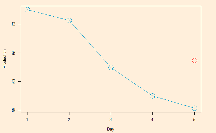
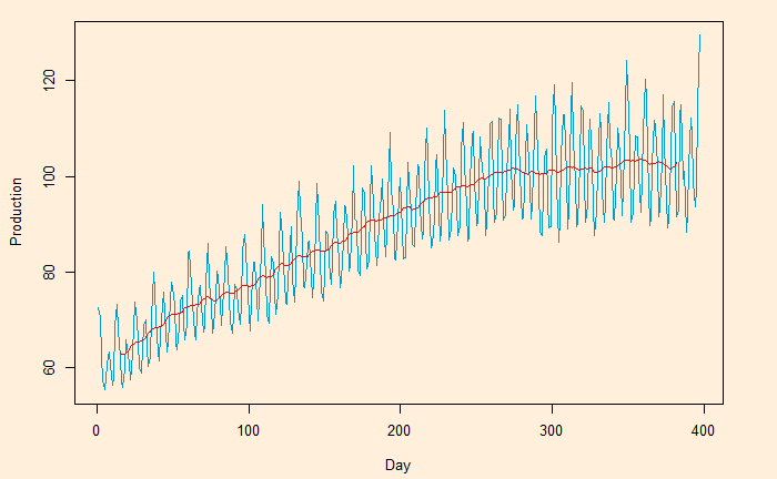
Here, we plot the daily electricity production data that was used in the last post.
Following is the R code, which uses the filter function for building the 2-sided moving average. The subsequent plot represents the method on the first five points (the red circle represents the centred average of the first five points).
Moving averages and means to smoothen noisy (time series) data, unearthing the underlying trends. The process is also known as filtering the data.
Moving averages (MA) are a series of averages estimated on a pre-defined number of consecutive data. For example, MA5 contains the set of all the averages of 5 successive members of the original series. The following relationship represents how a centred or two-sided moving average is estimated.
MA5 = (Xt-2 + Xt-1 + Xt + Xt+1 + Xt+2)/5
‘t’ represents the time at which the moving average is estimated. t-1 is the observation just before t, and t+1 means one observation immediately after t. To illustrate the concept, we develop the following table representing consecutive 10 points (electric signals) in a dataset.
Date
Signal
1
72.5052
2
70.6720
3
62.4502
4
57.4714
5
55.3151
6
58.0904
7
62.6202
8
63.2485
9
60.5846
10
56.3154
The centred MA starts from point 3 (the midpoint of 1, 2, 3, 4, 5). The value at 3 is the mean of the first five points (72.5052 + 70.6720 + 62.4502 + 57.4714 + 55.3151) /5 = 63.68278.
Date
Signal
Average
1
72.5052
2
70.6720
3
62.4502
63.68278
4
57.4714
5
55.3151
6
58.0904
7
62.6202
8
63.2485
9
60.5846
10
56.3154
This process is continued – MA on point 4 is the mean of points 2, 3, 4, 5 and 6, etc.
Date
Signal
MA
1
72.5052
2
70.6720
3
62.4502
63.68278 [1-5]
4
57.4714
60.79982 [2-6]
5
55.3151
59.18946 [3-7]
6
58.0904
59.34912 [4-8]
7
62.6202
59.97176 [5-9]
8
63.2485
60.17182 [6-10]
9
60.5846
10
56.3154
The one-sided moving average is different. It estimates MA at the end of the interval. MA5 = (Xt-4 + Xt-3 + Xt-2 + Xt-1 + Xt)/5
Date
Signal
MA
1
72.5052
2
70.6720
3
62.4502
4
57.4714
5
55.3151
63.68278 [1-5]
6
58.0904
60.79982 [2-6]
7
62.6202
59.18946 [3-7]
8
63.2485
59.34912 [4-8]
9
60.5846
59.97176 [5-9]
10
56.3154
60.17182 [6-10]
We will look at the impact of moving averages in the next post.
Now, we create a new variable, FAT (in kg), multiplying fat percentage with weight. First, we rerun the correlation to check how the new variables relate.
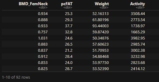
We have seen estimating the variance inflation factor (VIF) is a way of detecting multicollinearity during regression. This time, we will work out one example using the data frame from “Statistics by Jim”. We will use R programs to execute the regressions.
This regression will model the relationship between the dependent variable (Y), the bone mineral density of the femoral neck, and three independent variables (Xs): physical activity, body fat percentage, and weight. The first few lines of the data are below:
The objective of the regression is to find the best (linear) model that fits BMD_FemNeck with pcFAT, Weight, and Activity.
Call:
lm(formula = BMD_FemNeck ~ pcFAT + Weight + Activity, data = M_data)

Residuals:
      Min        1Q    Median        3Q       Max
-0.210260 -0.041555 -0.002586  0.035086  0.213329

Coefficients:
              Estimate Std. Error t value Pr(>|t|)
(Intercept)  5.214e-01  3.830e-02  13.614  < 2e-16 ***
pcFAT       -4.923e-03  1.971e-03  -2.498 0.014361 *
Weight       6.608e-03  9.174e-04   7.203 1.91e-10 ***
Activity     2.574e-05  7.479e-06   3.442 0.000887 ***
---
Signif. codes:  0 ‘***’ 0.001 ‘**’ 0.01 ‘*’ 0.05 ‘.’ 0.1 ‘ ’ 1

Residual standard error: 0.07342 on 88 degrees of freedom
Multiple R-squared:  0.5201,	Adjusted R-squared:  0.5037
F-statistic: 31.79 on 3 and 88 DF,  p-value: 5.138e-14
The relationship will be:
5.214e-01 – 4.923e-03 x pcFAT + 6.608e-03 x Weight + 2.574e-05 x Activity
To estimate each VIF value, we will first consider the corresponding X value as the dependent variable (against the remaining Xs as the independent variables), do regression and evaluate the R-squared.
The first thing that can be done is to find pairwise correlations between all X variables. If two variables are perfectly uncorrelated, the correlation is zero, one suggesting a perfect correlation. In our case, a correlation of > 0.9 must sound an alarm for multicollinearity.
Another method to detect multicollinearity is the Variance Inflation Factor (VIF). VIF estimates how much the variance of the estimated regression coefficients is inflated compared to when Xs are not linearly related. The way to estimate VIF work the following way:
Create an auxiliary regression for each X, such as X1 = A0 + A*1 X2 + A*2 X3 + … Or how much the X1 regresses using the other independent variables.
Estimate R-squared from the regression model
VIF (X1) = 1/(1-R21)
As a rule of thumb, a VIF of > 10 suggests that X is redundant in the original model.
Regression, as we know, is the description of the dependent variable, Y, as a function of a bunch of independent variables, X1, X2, X3, etc. Y = A0 + A1 X1 + A2 X2 + A3 X3 + …
A1, A2, etc., are coefficients representing the marginal effect of the respective X variable on the impact of Y while keeping all the other Xs constant.
But what happens when the X variables are correlated? – that is multicollinearity.
Finding the average of a set of values (of samples) is something we all know. Annie has 50 dollars, Becky has 30, and Carol has 10. What is the average amount of money they hold? You sum the numbers and divide by the number of sums, i.e., (50+30+10)/3 = 90/3 = 30. This is mean, but more specifically, the arithmetic mean.
Now look at this: I have invested 100 dollars in the market. It gave 10% in the first year, 20% in the second, and 30% in the third. What is the average annualised rate of return? The first instinct is to take the arithmetic mean of the three numbers and report it as 20%. Well, is that correct? Let’s check.
Money at the end of year 1 = 100 x (1.1) = 110 Money at the end of year 2 = 110 x (1.2) = 132 Money at the end of year 3 = 132 x (1.3) = 171.6
Now, let’s calculate the final amount using the proposed mean, i.e., 20%. The calculation led to 100x(1.2)3 = 172.8; not quite the same!
Here, we estimate the geometric mean by multiplying the returns and taking the cube root. Mean = [(1.1)x(1.2)x(1.3)]1/3 = 1.7163 = 1.197216; the average return is 0.1972 or 19.72%. The average return using the new (geometric) mean is 100x(1.197216)3 = 171.6.
Abby ran the first lap at 10 km/hr speed and the second at 12 km/hr. What is Abby’s average speed? The answer is neither (10+12)/2 nor (10×12)1/2. It is 2/(1/10 + 1/12) = 10.9. It is known as the harmonic mean and is given by:
We know standard deviation quantifies the spread of data from the mean. It is an absolute measure, and therefore, it has the same unit as the variable. However, it is limited when comparing two standard deviations of samples having different means. For example, compare the spread of the following two samples: the spending habits of two types of households.
Sample 1 (high income = mean income 400,000): standard deviation = 40,000 Sample 2 (low income = mean income 10,000): standard deviation = 1,000
It appears that the variability of data in the high-income category is higher. Or is it?
In such cases, non-dimensionalizing or standardization of the spread comes in handy. The Coefficient of Variation (CV) is one such. It is the ratio between the standard deviation and the mean. Since both possess the same unit, the ratio is dimensionless.
CV = Standard Deviation / Mean
Let’s calculate the CVs of sample 1 and sample 2. CV1 (high income) = 400,000 / 40,000 = 10 CV2 (low income) = 10,000 / 1,000 = 10
Anna must select seven classes out of the 30 non-overlapping courses. Each course happens once a week and is distributed equally from Monday through Friday (6 courses a week). What is the probability that she has courses every day (Monday through Friday)?


![\sqrt[n]{\Pi x}](https://thoughtfulexaminations.com/wp-content/ql-cache/quicklatex.com-fbf592781a23df1cd19d67b85addacdc_l3.png "Rendered by QuickLaTeX.com")

