Data & Statistics

Let’s apply what we learned in the ‘mtcars’ data. We use R to perform the calculations. We require two packages, ‘stats’ and ‘ggbiplot’, to do the job.

library(stats)
library(ggbiplot)

Start with the simplest first – two variables – mpg and disp

data("mtcars")
car_data <- mtcars
mtcars.pca <- prcomp(car_data[,c(1,3)], center = TRUE,scale. = TRUE)
ggbiplot(mtcars.pca,
  ellipse = TRUE,
  labels = rownames(car_data)
)

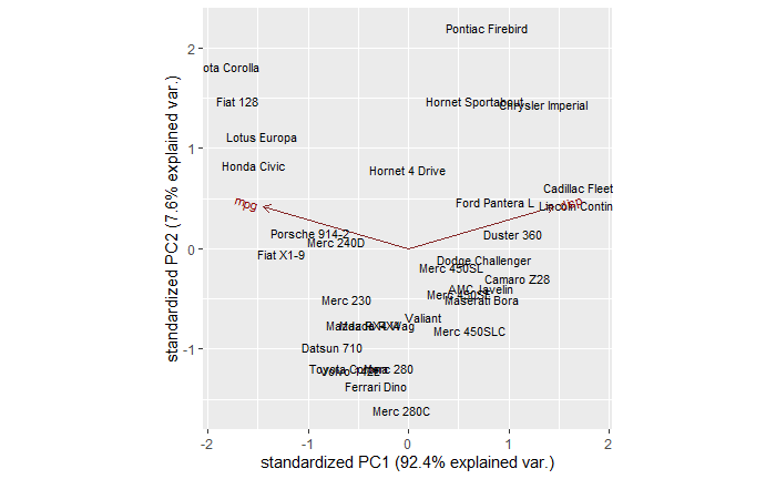
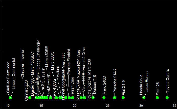
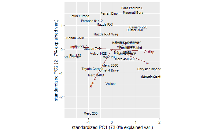
You can see a few clusters – things on the right, left and centre. You can also see two arrows, one corresponding to mpg and another to disp. It’s true we don’t need to do a PCA for two variables; a 2-D can do the job already.

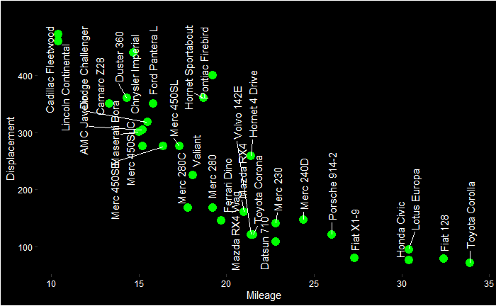
You can already start interpreting the PCA plot. The Cadilac and Lincoln are closer to the disp line in the PCA plot, which is towards the northwest of the Displacement vs Mileage plot. On the other hand, Honda, Porche etc., are closer to the mpg axis.

mtcars.pca <- prcomp(car_data[,c(1,3, 6, 7)], center = TRUE,scale. = TRUE)
ggbiplot(mtcars.pca)
ggbiplot(mtcars.pca,
  ellipse = TRUE,
  labels = rownames(car_data)#,
)

Last time we saw the practical difficulty of analysing data from four or more measured variables. The demands a means of reducing the numbers to two so that it appears on a 2-D plot but gives the message we want – that similar candidates cluster together.

In other words, one must perform necessary mathematical manipulations to convert the parameters to a different set of variables (principal components), select the top two or the principal components, and plot them. All these happen without losing much of the information embedded inside it.

PCA is the technique of compressing data from a large set of measurements into a smaller number of independent (i.e., uncorrelated) variables that captures the core of the original data. Note that the principal component themselves are linear combinations of the original variables.

The first principal component, which becomes the X-axis, defines the direction of the maximum variation of data.

Do you remember the “mtcars” dataset? It’s data collected from the 1974 Motor Trend US magazine and it comprises fuel consumption and ten aspects of automobile design and performance for 32 automobiles (1973–74 models). We’ll use it to explain the concept of principal component analysis or PCA.

If we measure only one aspect, we can present the data on a line plot:

You can see that Toyota Corolla, Fiat 128 etc., are similar to each other, and have relatively higher mileage values, whereas Cadillac Fleetwood and Lincoln Continental have lower.

If we measure two properties, we can present the data in a 2-D graph.

If we measure one more property, we would add one more axis to the graph for a 3-D plot. But what happens if we have four or more parameters? PCA can take four or more measurements and make a 2-D PCA plot.