Data & Statistics

Geometric Distribution

One in five cars in the city is green. What is the probability that the fifth car is the first green car?

We already know we can solve this problem using the negative binomial distribution function. But there is a special one for these types – where the arrival time of the first in question. That is the geometric distribution. The formal expression of the probability that the first occurrence of success requires k independent trials, each with success probability p is

\\ P(X = k) = p * (1-p)^{k-1}

To answer the question in the beginning, we substitute p = 0.20 (one in fifth), car number = 5; the required probability is (0.2)*(1-0.2)4 = 0.08192

The R code for the same calculation is
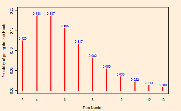
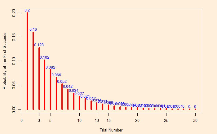
dgeom(4, prob = 0.2, log = FALSE)

The below geometric distribution chart shows the probability of seeing the first green car in precisely 1, 2, 3, etc. rolls, up to 30.

Geometric Distribution Read More »

Discrete Probability Distributions 

We have seen a few discrete probability distributions by now. Today we summarise them and find the relationships and the differences. The following are considered here:

Bernoulli distribution

The Bernoulli distribution is the distribution of the number of successes on a single Bernoulli trial. In a Bernoulli trial, you either get a success (1) or a failure (0). Therefore, a Bernoulli random variable can take either zero or one. E.g., if a coin is tossed once, what is the probability that it comes up heads?

Binomial distribution

When you carry out multiple Bernoulli trials, we get into a Binomial distribution. E.g., if I toss a coin ten times, what is the probability of getting exactly four heads? So, you can already conclude that the Bernoulli distribution is a special case of the binomial distribution with one trial.

Geometric distribution

The geometric distribution is the distribution of the number of Bernoulli trials to get the first success. E.g., if a coin is tossed repeatedly, what is the probability that the first head comes on the fifth trial?

Negative binomial distribution

A general case of the geometric distribution is the negative binomial distribution. It is the distribution of the number of trials needed to get a certain number of successes in repeated independent Bernoulli trials. E.g., if a coin is tossed repeatedly, what is the probability that the third head comes on the tenth trial?

Hypergeometric distribution

The hypergeometric distribution is similar to the binomial distribution but without replacement, or the trials are not independent. E.g., if five cards are drawn from a deck without replacement, what is the probability of getting two spades?

Poisson distribution

It is the distribution of the number of events in a given duration if those are occurring randomly and independently. What is the probability of having exactly three shark attacks on a particular beach this year? The Poisson distribution is approximated to a binomial distribution if the number of trials is large and the probability is small.

Reference

Overview of Some Discrete Probability Distributions: jbstatistics

Discrete Probability Distributions  Read More »

Negative Binomial Distribution

A fair coin is tossed repeatedly. What is the chance of getting 3rd head on the 10th toss?

You may notice the difference here; it is not asking for the probability of getting three heads in 10 tosses, which can be done using a binomial distribution. This one belongs to the negative binomial distribution.

Let each trial has a probability of success p (and failure 1−p). We follow this sequence until r successes occur.

The probability of observing the s success after having f failures (i.e., the success specified for the [s+f]th trial) is s+f-1Cf x ps x qf

The present problem

\frac{9!}{2! 7!} * (0.5)^3 * (1-0.5)^7 = 0.035

or the R – code

toss_number <- 10
success <- 3
failure <- toss_number - success
dnbinom(failure, success, prob = 0.5)
0.035

Here is the distribution of probabilities of success at each milestone.

Binomial and negative binomial

The key difference between the two is: in the binomial distribution, the number of trials is fixed and the number of successes is a random variable. Whereas in the negative binomial distribution, the opposite is true, viz. the number of successes is fixed and the number of trials is a random variable.

Negative Binomial Distribution Read More »

A pair of Aces from Four Cards

There are four cards – ace of spades, ace of clubs, ten of spades and seven of clubs.

A♠; A♣; 10♠; 7♣

If I draw two random cards, what is the probability that I get two aces, given?
1. At least one of them is an ace
2. One card is an ace of spades

The problem can be solved in different ways, but we choose, as usual, the Bayes’ rule.

At least one of them is an ace

\\ P(AA|A_{At1}) = \frac{P(A_{At1}|AA) * P(AA)}{P(A_{At1}|AA) * P(AA) + P(A_{At1}|AA^n)* P(AA^n)}

Estimating each parameter:
Probability of at least one Ace, given two aces, P(AAt1|AA) = 1
Probability of picking two aces, P(AA) = 1/6 (there are six ways of arranging four cards into pairs)
Probability of at least one Ace, given NOT two aces, P(AAt1|AAn) = 4/5
Probability of NOT picking two aces, P(AAn) = 5/6 [P(AA) + P(AAn) = 1]
Substituting the values,

\\ P(AA|A_{At1}) = \frac{1/6}{1/6 + (4/5)*(5/6)} = \frac{1}{1+4} = \frac{1}{5}

One card is an ace of spades

\\ P(AA|A_{Asp}) = \frac{P(A_{Asp}|AA) * P(AA)}{P(A_{Asp}|AA) * P(AA) + P(A_{Asp}|AA^n)* P(AA^n)}

Probability of Ace of Spades, given two aces, P(AAsp|AA) = 1
Probability of picking two aces, P(AA) = 1/6 (there are six ways of arranging four cards into pairs)
Probability of Ace of Spades, given NOT two aces, P(AAsp|AAn) = 2/5
Probability of NOT picking two aces, P(AAn) = 5/6 [P(AA) + P(AAn) = 1]
Substituting the values,

\\ P(AA|A_{Asp}) = \frac{1/6}{1/6 + (2/5)*(5/6)} = \frac{1}{1+2} = \frac{1}{3}

R Simulation

cards <- c("Ace of Spades", "Ace of Clubs", "Ten of Spades", "Seven of Clubs")

itr <- 100000

shuff <- replicate(itr, {
draw <- sample(cards, 2, replace = FALSE, prob = rep(1/4, 4)) 

if(any(str_detect(draw, "Ace of Spades"))) {
  if(all(str_detect(draw, "Ace"))){counter <- "A"}
  else{counter <- "B"}
}
else{counter <- "C"}
})

sum(shuff == "A") / (sum(shuff == "A") + sum(shuff == "B"))

A pair of Aces from Four Cards Read More »

Cards from a Deck

If you draw cards from a well-shuffled deck of cards, what is the probability that you get an Ace of Hearts and a black card?

There are two different probabilities this can happen.

  1. An ace of hearts followed by a black card
  2. A black card followed by an ace of hearts

The probability for 1) is (1/52) x (26/51) and for 2) is (26/52) x (1/51). Add them up: (2 x 26)/(51 x 52) = 1/51

If you want to verify the results, you may shuffle the deck a million times and count:

suits <- c("Diamonds", "Spades", "Hearts", "Clubs")
face <- c("Jack", "Queen", "King")
numb <- c("Deuce", "Three", "Four", "Five", "Six", "Seven", "Eight", "Nine", "Ten")
face_card <- expand.grid(Face = face, Suit = suits)
face_card <- paste(face_card$Face, face_card$Suit)

numb_card <- expand.grid(Numb = numb, Suit = suits)
numb_card <- paste(numb_card$Numb, numb_card$Suit)

Aces <- paste("Ace", suits) 

deck <- c(Aces, numb_card, face_card)
itr <- 1000000

shuff <- replicate(itr, {
draw <- sample(deck, 2, replace = FALSE, prob = rep(1/52, 52)) 

dr <- "Ace Hearts" %in% draw & (any(str_detect(draw, "Spades|Clubs")))

if(dr == TRUE){
  counter <- 1
}else{ 
counter <- 0
}

})

mean(shuff)

Cards from a Deck Read More »

The Climate Data – Nasa Power

NS_data <- get_power(
  community = "re",
  lonlat = c(1.6780, 56.5187),
  pars = c("T2M", "WS10M", "WD10M"),
  dates = c("2021-1-1", "2021-03-31"),
  temporal_api = "daily")

Wind_rose<-NS_data[,9:10]
colnames(Wind_rose)<-c("ws", "wd")

windRose(Wind_rose,paddle = FALSE,breaks = c(1,5,10,15,20),
         col=c("#4f4f4f", "#0a7cb9", "#f9be00", "#ff7f2f"))

References

The Power Project: NASA

The Climate Data – Nasa Power Read More »

Drinking and Police

Here is some data on drinking and getting in trouble with the police. Assess the relationship between drinking habits and getting into trouble with the authorities. Does this data provide evidence of drinking and getting into trouble with the police?

NeverOccasionalFrequent
Trouble with Police 60200420
No trouble with Police 480027002800
Observation table

The first step is to form the hypothesis. Here is the null hypothesis:

H0 – Drinking habits and getting into trouble with the police are independent.

The alternative is

H1 – Drinking habits and getting into trouble with the police are not independent.

We will use the chi-squared test to validate the null hypothesis.

We will use the chi-squared test to validate the null hypothesis. It requires observed data as well as the expected data under the null hypothesis conditions. From the data, the number of people belonging to each of the drinking categories is:

NeverOccasionalFrequentTotal
#48602900322010980
%44.2626.4129.33100

So, under ‘normal’ conditions (conditions of independence), one would expect similar percentages of individuals getting into trouble with the police, the expected numbers we needed.

NeverOccasionalFrequent
Trouble with Police 301178200
No trouble with Police 455927203020
Expectation table

If you add a row below each category, you will get the same split as per the total.

NeverOccasionalFrequent
%44.2626.4129.33

It’s time for the chi-square test, i.e. (observed – expected)2/expected summed over all the members.

(60 – 301)2 / 301 + (200 – 178)2 / 178 + (420 – 200)2 / 200 +(4800 – 4559)2 / 4559 +(2700 – 2720)2 / 2720 + (2800 – 3020)2 / 3020 = 467

The chi-squared statistic is 467. The degrees of freedom are the product of one less than the number of categorical variables (i.e. (2-1) x (3-1) = 2). Upon looking at the probability table, you can find that 467 is way on the right side of the distribution, with the probability (p-value) almost zero. So the data did not happen by chance, and the null hypothesis is rejected.

Drinking and Police Read More »

Portfolio Theory – Normal DIstribution

With all its simplicity, portfolio theory still describes the value in grouping securities, preferably ones uncorrelated with each other, for more predictable returns. The statistical parameters, mean and standard deviation, representing the expected return and risk, respectively, also suggest an underlying probability distribution. Despite all criticism around the usage or normal distribution (symmetric bell curve), we still utilise it to explain the portfolio concept.

In the previous post, we saw two stocks, 1 and 2, with two different expected returns (12 and 6) and risks (6 and 3). If the overall returns followed a normal distribution, they would have appeared like in the following plot.

Here, the blue curve represents the one with a higher expected return and higher volatility. The red one is more conservative. The combined set (1:1) for a correlation coefficient of 0 (uncorrelated) behaves in the following way.

The advantage of using a standard distribution (normal, in this case) is that it enables us to estimate various probabilities. E.g., the chance of ending up with a zero return and below for the blue curve (aggressive one) is 2.3%, which is similar to what the conservative (red) can give. On the other hand, for the joint distribution (green curve), it is just 0.4%.

Portfolio Theory – Normal DIstribution Read More »

Portfolio Theory

Portfolio theory is a simple theoretical framework for building investment mixes to achieve returns while managing risks. It used the concepts of expected values and standard deviations to communicate the philosophy.

Take two funds, 1 and 2. 1 has an expected rate of return of 12%, and 2 has 6%. On the other hand, 1 is more volatile (standard deviation = 6), whereas 2 is less risky (standard deviation = 3), based on historical performances. In one scenario, you invest 50:50 in each.

The expected value is 0.5 x 12 + 0.5 x 6 = 9%

To estimate the risk of the portfolio, construct the following matrix.

Omega values (1 and 2) are the proportions, sigmas are the standard deviations, and sigma12 is the covariance between 1 and 2. Substituting 0.5 for each omega (50:50) and noting that covariance is the product of the standard deviations x correlation coefficient, we get the following table for the two securities that are weakly correlated (correlation coefficient = 0.5),

Add the entries in these boxes to get the portfolio variance. Take the square root for the standard deviation = 3.97.

The expected rate of return of the portfolio is 9%, and the risk (volatility) is 3.97%. Continue this for all the proportions (omega1 = 1 to 0) and then plot the returns vs volatility; you get the following plot for a correlation coefficient of 0.5.

Imagine the securities do not correlate (coefficient = 0). The relationship changes to the following.

The risk is lower than the lowest (3%) for proportions of security1 less than 0.4. Even better, if the two securities are negatively correlated (correlation coefficient = -0.5),

If there are n securities in the portfolio, you must create an n x n matrix to determine the variance.

Portfolio Theory Read More »

Bayes’ Theorem – Graphical Representation

Here is a graphical illustration of Bayes’ theory. We use the old example of Steve, “the shy and withdrawn”.

The colour orange represents the number of librarians, and the light blue the farmers.

From the relative sizes of the rectangles, you make out that the number of farmers is more than the number of librarians. This, we call, the prior information.

Let’s assume that 80% of the librarians are shy and withdrawn, and only 25% of the farmers possess those characteristics. The following picture, green representing shyness, is more or less that.

Now, here is the question: when you see a random shy and withdrawn person, where do you likely to classify him, given you have two choices – librarian or farmer?

Well, likely in the rectangle on the left, which comes from the farmer group! And if you want a precise probability, here is the math below:

Bayes’ Theorem – Graphical Representation Read More »