Period Life Expectancy – Plots

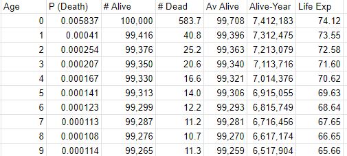
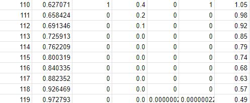
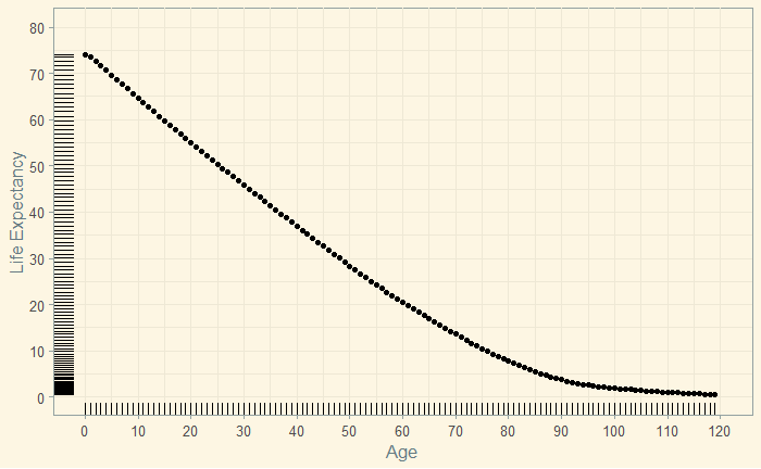
We have seen the calculations behind life expectancy, the lifespan of a hypothetical cohort ageing based on the measured mortality rates of a given period, as a statistical projection of the current conditions. Here, we plot the life expectancy that we estimated previously.

library(tidyverse)
library(ggthemes)
L_data %>% ggplot(aes(Age, Life.Exp)) +
geom_point() +
   geom_rug() +
  scale_x_continuous(name="Age", limits=c(0, 120), minor_breaks = seq(0, 120, 5), breaks=seq(0, 120, 10)) +
  scale_y_continuous(name="Life Expectancy", limits=c(0, 80), minor_breaks = seq(0, 80, 5), breaks=seq(0, 80, 10)) + 
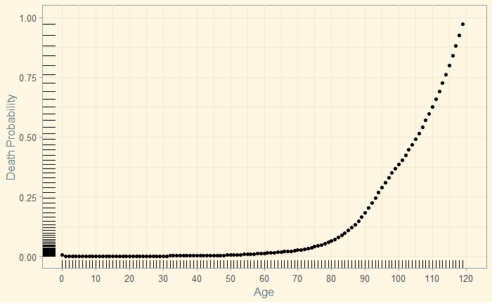
 theme_solarized(light = TRUE) 

The death probability (data) at each age is presented below.

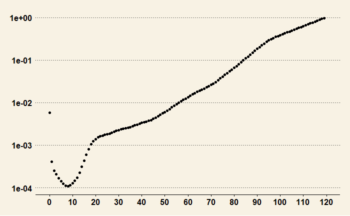
The plot with the Y-axis in the logarithmic scale shows finer details, especially in the lower age categories.

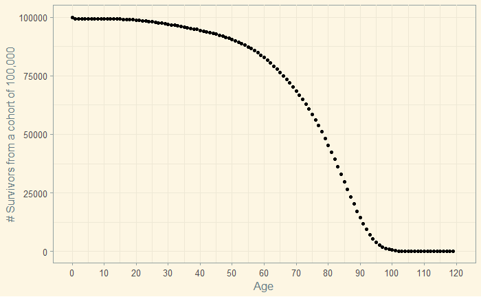
You can see below the dynamics of survival – 85,000 of the 100,000 are alive until almost the age of 60.

Period Life Expectancy – Plots Read More »

Period Life Expectancy

The period-life expectancy at a given age is the average remaining number of years expected for a person at that exact age, estimated from the mortality rate of that particular time. Let’s work out the calculation using the death probability (probability of dying within one year) table. The death probability is estimated from the mortality rates at each age (from census data for a short period). Here are the first few lines of the data (for complete data, see reference).

AgeP (Death)
00.005837
10.00041
20.000254
30.000207
40.000167

We start with 100,000 people in the cohort. The number of deaths in a given year, Yx = the probability of death (in Yx) x people alive (in Yx). In our example, for Y1, it is 100,000 x 0.005837 = 583.7.

The number of people alive in the next year (Yx+1 ) = people alive (in Yx) – the number of deaths in a given year (x). I.e., # Alivex+1 = 100,000 – 583.7 = 99,416. This number multiplied by the probability gives the number of dead in Yx+1.

The next step is to calculate the average number of people alive in the age category. It can be calculated as a mid-point average of the number of people in Yx+1 + (1/2) of the death in Yx. That equals 99,416 + 0.5 x 583.7 = 99,708.

In the next step, the total number of person-years lived by the cohort from age x until all cohort members have died. It is the sum of the numbers in the mid-point average column from age x to the last row in the table. Suppose there are a total of 120 columns (age numbers), and you want to calculate the person-years of age 24, you add all average alive from Y24 till Y119.

Life expectancy for a given age = person-years / persons alive.

Here are the first and the last 10 years of calculations of a table that has 120 rows (Y0 – Y119).

References

Actuarial Life Table: SSA

The Life Table: lifeexpectancy.org

Period Life Expectancy Read More »

Likelihood Ratio – Fagan’s Nomogram

We have seen the likelihood ratio as the property of a diagnostic tool. Let’s take the fictitious screening tool we evaluated in the last post with LR+ = 10.7. Imagine a patient comes to a clinic with a few symptoms of a disease with a prevalence of 0.1 (very likely, age-adjusted), and this screening is a possible option. Would you recommend this? Note that the doctor will decide on further (costly) treatment only if she gets a conformation (posterior probability) of > 50% chance of the disease.

From the relationship we derived last time, 

OR_Post = LR x OR_Pri

Odds ratio (posterior) = 10.7 x 0.11 = 1.07
P(poterior) / (1 – P(poterior)) = 1.88
1/P(poterior) = 1 + 1/1.88
P(poterior) = 1.88/2.88 = 0.54

A nomogram of the following type is built to make such calculations simpler.

Draw a line from the ‘pre-test probability’ to ‘the likelihood ratio’ and extend it to the ‘post-test probability line. The intersection gives the posterior probability.

Here is an illustration of the method. Let’s use Fagan’s nomogram for the previous case,

To answer the original question: this test may be recommended as it can bring the probability over 0.5 if the test comes positive. Not to forget, if the test comes negative (LR- = 0.044), the posterior probability becomes 0.005.

Smaller prior

On the other hand, if the prior probability is lower, say, 0.01, as you can see below, the test is not very useful to make a conclusive decision.

Such a disease would require a diagnostic tool with a likelihood ratio of 100 or above to make a decision. Connect 0.01 (prior probability) to 0.5 (minimum decision criterion) and find out the likelihood ratio.

Likelihood Ratio – Fagan’s Nomogram Read More »

Likelihood Ratio and Posterior Odds

We know how the updated (posterior) disease probability is related to the prevalence (prior) via Bayes’ relationship.

\text{Posterior} = \frac{Sensitivity *  Prior}{Sensitivity *  Prior + (1-Specificity)*(1- Prior)}

Here, the ‘posterior’ and ‘prior’ are probability values. The corresponding odds ratio may be calculated using the following formula,

\text{Odds Ratio} = \frac{P}{1-P}

Using this definition, we estimate the odds ratio of the posterior as:

\\ OR_{post}= \frac{Posterior}{1-Posterior} \\ \\ = \frac{\frac{Sensitivity *  Prior}{Sensitivity *  Prior + (1-Specificity)*(1- Prior)}}{1 - \frac{Sensitivity *  Prior}{Sensitivity *  Prior + (1-Specificity)*(1- Prior)}} \\ \\ = \frac{Sensitivity *  Prior} {(1-Specificity)*(1- Prior)} = \frac{Sensitivity} {(1-Specificity)}\frac{Prior}{(1- Prior)}}

Notice the two terms: the first term, Sensitivity / (1 – Specificity), is the likelihood ratio and the second term, Prior / (1-Prior), is the odds ratio of the prior. Therefore,

OR_Post = LR x OR_Pri

Example

A new diagnostic tool yielded the following results.

  • A total of 1,000 individuals took the test.
  • 435 individuals had positive results, and 565 were negative.
  • Out of the 435 positive, 381 of them had the disease.
  • Out of the 565 negative, 549 did not have the disease.

What is the positive likelihood ratio of the test method?

From the data, true positives (TP) are 381. Then 435 – 381 = 54 must be false positives (FP).
Similarly, the true negatives (TN) are 549. 565 – 549 = 16 must be false negatives (FN).

Sensitivity = TP/(TP + FN) = 381/(381+16) = 0.96
Specificity = TN/(TN+FP) = 549 / (549 + 54) = 0.91

The likelihood ratio, therefore, is,
0.96 / (1 – 0.91) = 10.7

Likelihood Ratio and Posterior Odds Read More »

Likelihood Ratio

The likelihood ratio is the proportion of people with a disease and a test result vs. people without the disease and the same test result. In other words,

P(+ve AND D) / P(+ve AND D-) = P(TP) / P(FP) = [TP/TP+FN] / [FP/FP+TN]
LR+= Sensitivity / 1 – Specificity.

This is the positive likelihood ratio (LR+)

In the same way, there is a negative likelihood ratio (LR-),
P(-ve AND D) / P(-ve AND D-) = P(FN) / P(TN) = TP/TP+FN
LR- = (1-Sensitivity) / Specificity

Note that both these ratios don’t depend on the prevalence of the disease but on the measurement techniques. A likelihood ratio of close to 1 means that the particular test has little influence on determining whether the patient has the suspected condition or not. Likelihood ratios > 10 and < 0.1 are considered to provide robust evidence for and against the diagnoses, respectively.

Likelihood Ratio Read More »

Two-Proportions Z-Test

A survey revealed the following information on the prevalence of eye disease. Check if the difference in prevalence is statistically significant.

ResidenceEye DiseaseTotal
YesNo
Rural24276300
Urban15485500

z = \frac{p_1 - p_2}{\sqrt{p_1(1-p_1)/n_1 + p_2(1-p_2)/n_2}}

n1: sample size of population 1 = 300
n2: sample size of population 2 = 500
p1: sample proportion for population 1 = 24/300
p2: sample proportion for population 2 = 15/500

z = \frac{0.08 - 0.03}{\sqrt{0.08(1-0.08)/300 + 0.03(1-0.03)/500}} =  2.87

Critical z = 1.96 at a 5% confidence interval.
Therefore, z = 2.87 > critical z; the difference in prevalence of eye disease between urban and rural is significant.

Two-Proportions Z-Test Read More »

Enigmatic Possibilities

The Enigma machine was an electromechanical device built by the Germans in World War II to mechanise encryption. The device was about the size of a typewriter and had two sets of letters on a keyboard and a lampboard. The message got encrypted letter by letter.

The Enigma machine was a large circuit. It had the following components.

  1. Rotors 1, 2, and 3. They connected the cris-cross wires from one letter to another. But these three rotors are selected from a total of five.
  2. The reflector connected 26 letters into 13 pairs.
  3. The plugboard connected some letters into pairs, and some were left unconnected. In one version, it connected 20 letters into ten pairs and left six unpaired.

So what are the total possibilities?

1) 3 chose from 5 (and order matters) => 5!/2! = 60.
2) Three rotors with 26 letters available => 26 x 26 x 26 possibilities
3) 10 pairs from 26 possible letters => 26!/6!10!210. 210 comes because a pair AB is indistinguishable from BA, and there were 10 such combinations.

Multiply all three, and you get the possible ways to set the enigma machine! That equals 1.589626e+20.

158,962,555,217,826,360,000 (Enigma Machine): Numberphile

Enigmatic Possibilities Read More »

Risk Preferences

We will use utility curves to illustrate three different kinds of risk preferences. They are:

Risk-averse

Here is a person who has the diminishing utility of marginal wealth. I.e., the extra dollar additional income from 10,000 to 10,001 brings a lesser increase in happiness to her than going from 100 to 101.

Notice the probabilistic (expected) utility line (blue) is below the certainty (brown).

Risk neutral

This person shows constant marginal utility. The person has the same happiness with a 1 dollar salary rise whether her current is at 10,000 or 100,000.

Risk lover

Imagine someone needs 100,000 for a major surgery to save her life. Smaller numbers don’t make much sense to her, and she is willing to gamble for a larger prize. She has increasing marginal utility.

Unsurprisingly, the expected utility line (blue) is above the certainty (brown).

Risk Preferences Read More »

Pascal’s Wager

Think about this game. There is a 1 in 1000 chance of winning a prize of 1 billion. The price of the ticket is $1. Will you take the gamble? Definitely, it is a good deal to buy the ticket. You only lose a dollar but get a chance to win a billion (expected value of a million).

Pascal used a similar argument to state that belief in god was a better deal than not doing so. He argues:
Proposition 1: God exists
Proposition 2: God doesn’t exist
If god exists and you believe, the payoff is infinitely good
If god exists and you don’t believe, the payoff is much worse
On the other hand, if god doesn’t exist, regardless of whether you believe in it or not, the payoffs (positive and negative) are finite. So, he argues, believing is a better deal.

God exists (G)God
does not exist (¬G)
Belief (B)infinite gainfinite loss
Disbelief (¬B)infinite lossfinite gain

Based on the payoff matrix, there is only one rational (!) decision: choose B.

Pascal’s wager: Wiki
PHILOSOPHY – Religion: Pascal’s Wager: Wireless Philosophy

Pascal’s Wager Read More »

The Probability of Steroid Team

A country has two teams of weightlifters; in one, 80% use steroids regularly, and in the other, only 20% use them. The head coach flips a coin and selects the team for the international meet. At the venue, if one lifter was selected at random for the drug test and found positive, what is the probability that the team is the steroid one?

We will use the base form of Bayes’ theorem – the relationship between conditional and joint probabilities.

P(S/T) = P(S & T) / P(T)
S – it is a steroid team
T – tested member used steroid
C – it is a clean team

P(S & T) = P(S) x P(T|S) = 0.5 (coin toss) x 0.8 (chance of using steroids, given he is from the steroid team) = 0.4
P(T) = P(S) x P(T|S) + P(C) x P(T|C) = 0.5 x 0.8 + 0.5 x 0.2 = 0.5
P(S/T) = 0.4/0.5 = 0.8

The probability that the team is the steroid one is 80%

The Probability of Steroid Team Read More »