Margin of Error – Continued

In the previous post, we saw how the margin of error at a specified confidence interval is estimated. The margin of error, and thereby the confidence in the data, varies with the number of samples and the confidence interval.

Here are five calculations with varying numbers of samples (500, 1041 and 2000) for three confidence intervals (90%, 95%, 99%).

As the sample size increases, the margin of error decreases, i.e., the more people you survey, the more confident you can be that your results are closer to the “true” population value (provided the sample is representative). However, the reduction diminishes as the sample size goes beyond 1000.

Margin of Error – Continued Read More »

Margin of Error

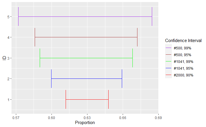
A recent study suggests that 63% of the people in a city believe in parapsychological phenomena. The study surveyed 1041 residents. What is the margin of error of the results at a 95% confidence interval?

This is the problem of estimating the margin of error on point estimates from a sample. You may know by now that the ultimate goal is to calculate the population proportion, for which sampling (and thus obtaining the sample proportion) is the only practical path. The point estimate of proportion, p, is evaluated from x, the number of successes (people who said “YES” to parapsychology here), and the sample size (n):
p = x/n

The remaining, 1 – p, is the proportion of failures (n – x out of n).

In the given sample, 0.63 is the p or the proportion of people who believed in parapsychology. Can you conclude that 0.63 remains the fraction of similar believers in the city? The answer is No; therefore, we estimate the margin of error by applying the formula. The margin of error gives the expected range of values to capture the population at some confidence level.

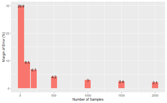
margin of error = z-critical value x square root (p x (1-p) / n)

MoE = z_{\alpha/2} \sqrt{\frac{p (1-p)}{n}}

z-critical value for a 95% confidence interval is 1.96, for 99% is 2.576, etc.

The whole process can be done in one step using R.

prop.test(proportion*n_sample, n_sample, p = NULL, alternative = "two.sided",
          correct = TRUE, conf.level = 0.95)
	1-sample proportions test with continuity correction

data:  proportion * n_sample out of n_sample, null probability 0.5
X-squared = 69.853, df = 1, p-value < 2.2e-16
alternative hypothesis: true p is not equal to 0.5
95 percent confidence interval:
 0.5997570 0.6592715
sample estimates:
   p 
0.63 

Or by applying the formula directly.

n_sample <- 1041
proportion <- 0.63

std_error <- sqrt(proportion*(1-proportion)/n_sample)
margin <- std_error*qnorm(0.975)
proportion + margin
proportion - margin

The margin of error is 0.029, and the confidence interval is found by adding and subtracting it from the sample proportion (0.63).

[ 0.600, 0.659]

So, we are 95% confident that the true proportion of the population lies between 0.600 and 0.659, right? Not really; it only means that if you perform several random samples from this population, we expect about 95% of those intervals to contain the true proportion.

Margin of Error Read More »

Anthropic Principle

The anthropic principle says that in the universe, our presence as observers compels conditions for our presence. While the idea was not entirely new, the phrase came up in 1973 by Brandon Carter, who proposed the weak and strong forms of anthropic principle.

The weak anthropic principle (WAP) merely says that you need to take into account those things in the environment that you can see vs those things you are unable to see. Or it simply says that the life-free universes cannot be observed it’s just a selection bias.

An example is the cosmological constant (lambda). The number must be within certain limits. If the constant were large-negative, the universe would have collapsed long ago; if it were large-positive, it would have expanded too fast for the stars to form. Either way, we wouldn’t be here to talk about it.

Anthropic Principle Read More »

Gambler, Learner and Logician

Amanda, Becky and Carol are at a betting station near the coin-flipping game. They observe five tosses and see all of them landing on heads.

Amanda: “It landed five times on heads; a tail is due, and I will bet on tails this time.
Becky: “It is a bised coin. The probability for the next flip to land on heads is high; I will bet on heads.
Carol: “Amanda has committed a fallacy. Becky may be right, but induction based on the first five tosses can still be logically incorrect. So there is no point betting either way”.

Who is right here?

Amanda has committed the Gambler’s fallacy. By expecting a tails due, she forgets about the independence of the trials.
Becky’s stand is based on her interpretation of the observations. Her argument is still not logically water-tight. From the casino’s point of view, using a biased coin is risky; people like Becky will find it easily and become rich.
In the absence of strong evidence, Amanda’s logic is more acceptable.

Gambler, Learner and Logician Read More »

Dieing to Fill Glasses

Here is a game: There are six empty glasses – numbered 1 through six. You roll a die and fill an empty glass that matches the die roll. If the number on the die matches with an already-filled glass, it will be emptied. How many rolls are required to fill all six glasses?

Suppose there are five filled glasses, the number of die rolls required before the game ends is denoted by E(5). Based on this definition, E(0) must be the number of die rolls to finish the game starting with 0 filled glasses, equivalent to the original question.

E(5) = (1/6)[1] + (5/6)[1 + E(4) ]

E(4) must be in the following form to extend the logic.
E(4) = (2/6)[1 + E(5)] + (4/6)[1 + E(3) ]
E(3) = (3/6)[1 + E(4)] + (3/6)[1 + E(2) ]
E(2) = (4/6)[1 + E(3)] + (2/6)[1 + E(1) ]
E(1) = (5/6)[1 + E(2)] + (1/6)[1 + E(0) ]
E(0) = (6/6)[1 + E(1)]

Solving the five equations with five unknowns,

E(0) = 83.2

Reference

Can You Solve The Dice Rolling Drinking Game?: MindYourDecisions

Dieing to Fill Glasses Read More »

Contingency Tables – Continued

Contingency Tables are one way to organise data. Here is a data summary of computer users in a group.

PCMacRow
Totals
Male453883
Female405595
Column
Totals
8593178

Joint Probability

What is the joint probability of Female and Mac?
First, the answer: go to the cell at the junction of Female and Mac, i.e., 55 and divide by the total. 55/178 = 0.309.

Now the theory:
P (F AND Mac) = P(F | Mac) x P(Mac)
P(F | Mac) = 55/93
P(Mac) = 93/178
P (F AND Mac) = (55/93) x (93/178) = 55/178 = 0.309.

PCMacRow
Totals
Male45/178
= 0.25
38/178
= 0.21
Female40/178
= 0.22
55/178
= 0.31
Column
Totals

Conditional Probabilities

Conditional probability is the probability that an event occurs, given another event has happened. Given that a customer is female, what is the probability she’ll purchase a Mac?

The answer is female-Mac cell (55) and divide it with the female row total (95). 55/95 = 0.58.

PCMacRow
Totals
MaleP(P|M)
45/83
P(M|M)
38/83
83
FemaleP(P|F)
40/95
P(M|F)
55/95
95
Column
Totals
8593178
PCMacRow
Totals
MaleP(M|P)
45/85
P(M|M)
38/93
83
FemaleP(F|P)
40/85
P(F|M)
55/93
95
Column
Totals
8593178

Contingency Tables – Continued Read More »

Contingency Tables

Contingency Tables are one way to organise data. Here is a data summary of computer users in a group.

PCMacRow
Totals
Male453883
Female405595
Column
Totals
8593178

The intersection between the row and column defines one piece of information. For example, The intersection of PC and Male, 45, is the number of males (who participated in the survey) who use a PC at work, the junction between row total and females (95) is the total number of females in the survey, and a total of 178 people in the study, etc.

Marginal, Joint, and conditional probabilities 

Before we get into the calculations, a gentle reminder on probability.
P(event) = # Events / # Outcomes.

Marginal probabilities are the probabilities for single events without counting the other events in the table.
P(Female) = # Females / # Grand Total = 95 / 178 = 0.53.
P(Mac sold) = # Mac / # Grand Total = 93/178 = 0.52.

Let’s redraw the contingency table with marginal probabilities now.

PCMacRow
Totals
Male83/178
0.47
Female95/178
0.53
Column
Totals
85/178
0.48
93/178
0.52
178/178
1.0

Clearly, the numbers are all sitting on the margins, hence the name.

We’ll see the other two probabilities in the next post.

Reference

Statistics By Jim: Page

Contingency Tables Read More »

Chi-Square Distribution

Chi-Square is a family of continuous distribution, widely used in hypothesis tests. The shape of a chi-square distribution is determined by what is known as the degree of freedom (df).

A chi-square test operates by comparing the observed distribution to what you expect if there is no relationship between the categorical variables.

Chi-Square Distribution Read More »

Likelihood Function – Part II

In the previous post, we estimated the likelihood of getting six people sick for two parameters (prevalence), 7% and 8%. We can also calculate the ratio between the two likelihoods:

L(theta = 0.07 | data = 6) / L(theta = 0.08 | data = 6) = 0.153 / 0.123 = 1.24. 

It means that the prevalence of 7% supports the data 1.24 times more than the prevalence of 8%. What about a sweep of likelihood over the entire parameter space? The function that gives the distribution of likelihoods of all possible values of parameters for a given data is the likelihood function.

As the parameter (theta) defines a model (e.g., binomial probability mass function), what the likelihood function is telling us is, given I have this data, what is the chance that the given model is true? In other words, we want the model that is mostly to have produced our data.

Likelihood Function – Part II Read More »

Likelihood Function

Consider two possible prevalence values for a rare disease, 0.07 and 0.08, respectively. If 100 samples from each city are taken, and six people are found positive, which prevalence value is likely?

Let’s visualise the situation 1:

And the situation 2:

It is clear that the first possibility, the prevalence (‘the parameter’) 0.07, is more likely, given 6 people tested positive as probability = 0.153 for the first case is > 0.123 for the second.

Summarising: for the parameter of 7%, the probability of getting six out of a hundred is 0.153. It becomes the likelihood.
L(theta = 0.07; y = 6) = 0.153 and L(theta = 0.08; y = 6) = 0.123

Here is the R code that generated the plot in situation 2.

xx <- seq(1,20)
P <-  dbinom(xx, 100, prob = 0.08)
binom_data <- data.frame(xx, P)

binom_data %>%  ggplot(aes(x=xx, y=P, label=P, fill=factor(ifelse(xx==6,"Highlighted","Normal")))) +
  geom_bar(stat="identity", show.legend = FALSE) +
  geom_text(aes(label=factor(ifelse(P > 0.01, round(P, 3),"")))) +
  scale_x_discrete(name = "Positive Sample", limits=factor(seq(1, 20, 1))) +
  scale_y_continuous(name = "Probability") +
  theme_solarized(light = TRUE) 

Likelihood Function Read More »