Shapiro-Wilk test – Test for Normality

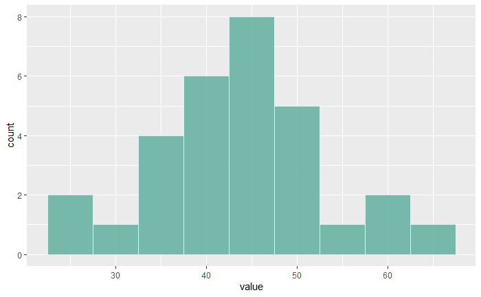
In the last post, we used a non-parametric hypothesis test, the Wilcoxon Signed Rank test. The p-value showed that the evidence was not sufficient to reject the null hypothesis. However, the histogram suggests that the data was reasonably a normal distribution.

Shapiro-Wilk test is a formal way of testing whether the data follows a normal distribution or not. The test has a null hypothesis that the sample comes from a normally distributed population. The test statistics, W has the following formula:

W = \frac{(\sum a_i x_i)^2}{\sum(x_i - \bar{x})^2}

We can apply the Shapiro-Wilk test to our data using the following R code:

diab <- c(35.5, 44.5, 39.8, 33.3, 51.4, 51.3, 30.5, 48.9, 42.1, 40.3, 46.8, 38.0, 40.1, 36.8, 39.3, 65.4, 42.6, 42.8, 59.8, 52.4, 26.2, 60.9, 45.6, 27.1, 47.3, 36.6, 55.6, 45.1, 52.2, 43.5)

shapiro.test(diab)
	Shapiro-Wilk normality test

data:  diab
W = 0.98494, p-value = 0.9361

The p-value is quite high, and the null hypothesis is not rejected. The same conclusion may be obtained by doing a q-q plot as follows.

qqnorm(diab)
qqline(diab, col = "darkgreen")

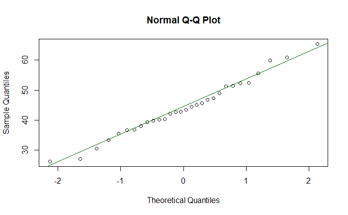
Shapiro-Wilk test – Test for Normality Read More »

Wilcoxon Signed Rank Test – R Program

We will use R to perform the hypothesis test using the Wilcoxon Signed Rank Test.

The expected median age for the onset of diabetes is 45 years. The following is a list of 30 people tracking their onset of diabetes. Test whether the evidence supports the hypothesis.

diab <- c(35.5, 44.5, 39.8, 33.3, 51.4, 51.3, 30.5, 48.9, 42.1, 40.3, 46.8, 38.0, 40.1, 36.8, 39.3, 65.4, 42.6, 42.8, 59.8, 52.4, 26.2, 60.9, 45.6, 27.1, 47.3, 36.6, 55.6, 45.1, 52.2, 43.5)

The Null Hypothesis, H0: Median equals 45
The Alternate Hypothesis, H1: Median does not equal 45

wilcox.test(diab, mu = 45.0, alternative = "two.sided")
	Wilcoxon signed rank exact test

data:  diab
V = 200, p-value = 0.5158
alternative hypothesis: true location is not equal to 45

The p-value is 0.51, which is higher than 0.05 (5% significance), and therefore, the null hypothesis can not be rejected.

Since the histogram of the data appears reasonably normal, it would be interesting to test using the parametric method, such as the t-test.

t.test(diab, mu = 45.0, alternative = "two.sided")
	One Sample t-test

data:  diab
t = -0.54461, df = 29, p-value = 0.5902
alternative hypothesis: true mean is not equal to 45
95 percent confidence interval:
 40.51408 47.59925
sample estimates:
mean of x 
 44.05667 

Wilcoxon Signed Rank Test – R Program Read More »

Wilcoxon Signed Rank Test

We continue with the same dataset but use another type of non-parametric test – the Wilcoxon Signed Rank Test. Here, not only the sign of the observation counts but also the distance of departure from the median.

Case #Drug A
112.3
213.1
311.3
410.1
514.0
613.3
710.5
812.3
910.9
1011.9

The Null Hypothesis, H0: Median = 13.0
The Alternate Hypothesis, H1: Median < 13.0

Steps

  1. Estimate the difference from the null hypothesis (median = 13.0)
  2. Calculate the absolute value
  3. Estimate the rank of the list, with the smallest absolute difference getting the lowest rank
  4. Add the sign (from the difference of step 1) to the rank
  5. Add all positives and negatives separately.
  6. Take the smaller of the two and check against the table of critical values.
Drug ADifferenceAbs
Difference
RankSigned
Rank
12.3-0.70.73.5-3.5
13.10.10.111
11.3-1.71.77-7
10.1-2.92.910-10
14.01.01.055
13.30.30.322
10.5-2.52.59-9
12.3-0.70.73.5-3.5
10.9-2.12.18-8
11.9-1.11.16-6

The sum of positive ranks = 8

The sum of negative ranks = 47

We’ll take the smaller, 8 and check against the table. The number in the table (n = 10, one-sided test, alpha = 0.5) is 10. Since 8 is smaller than 10, we reject the null hypothesis.

Non-parametric tests: zedstatistics

Wilcoxon Signed Rank Test Read More »

The sign test – Continued

The sign test is a simple non-parametric test. In the last example, we went for the median of a group, classified people as + or – based on the null hypothesis and evaluated the p-value.

Here are 10 individuals undergoing a particular diet. Their haemoglobin levels are measured. Note that levels below 13.0 g/dL qualify a person as anaemic. What is your conclusion regarding the possibility of this diet inducing anaemia?

Case #Drug A
112.3
213.1
311.3
410.1
514.0
613.3
710.5
812.3
910.9
1011.9

Our task is to assess whether the group’s median haemoglobin level is 13.0 or below. Needlessly, at a specified significance level, say at 5%.
The Null Hypothesis, H0: Median = 13.0
The Alternate Hypothesis, H1: Median < 13.0

Let’s re-draw the table after including the +/- convention – plus for > 13.0 and minus for < 13.0.

Case #Drug ASign
112.3
213.1+
311.3
410.1
514.0+
613.3+
710.5
812.3
910.9
1011.9

A person unexposed to statistics and random variations may conclude that at least five observations are required above 13.0 for the null hypothesis to be valid. And since there are only three, the null hypothesis is rejected. But we know about randomness and distributions, and therefore, ask this question: What is the probability of having seven negative observations from a binomial trial that is expected to have a 50% chance of success?

P(>=7) = P(7) + P(8) + P(9) + P(10) = 0.117 + 0.044 + 0.0098 + 0.001 = 0.172. In the following figure, it is the sum of the heights of the red bars.

So, the observations are unable to reject the null hypothesis. Before we end, answer this question: How many observations must be below 13.0 for the null hypothesis to be true? 

From the numbers and figure, it appears that you may need nine or ten observations below 13.0 for the sign test to make a rejection.

Does the magnitude of departure (from the median) play any role in rejecting the null hypothesis? We may have to explore another non-parametric test method, Wilcoxon signed rank, for that.

Non-parametric tests: zedstatistics

The sign test – Continued Read More »

The sign test

We have seen the definition of a non-parametric hypothesis test. The sign test is an example. We want to test the effectiveness of a drug from 12 observations. The data is the number of hours that the drug relieves pain. The null hypothesis is that the difference between paired medians equals zero.

Case #Drug ADrug B
12.03.5
23.65.7
32.62.9
42.62.4
57.39.9
63.43.3
714.916.7
86.66.0
92.33.8
1024.0
116.89.1
128.520.9

The paired differences (Drug B – Drug A) are:

data <- c(1.5, 2.1, 0.3, -0.2, 2.6, -0.1, 1.8, -0.6, 1.5, 2.0, 2.3, 12.4)

Let’s order them in the increasing magnitude.

sort(data) 
-0.6 -0.2 -0.1  0.3  1.5  1.5  1.8  2.0  2.1  2.3  2.6 12.4

Under the null hypothesis, we expect half the numbers to be above zero (median) and half below. Suppose r+ observations are > 0 and r < 0, then under the null hypothesis, r+ and r follow a binomial distribution with p = 1/2.

In our case, three cases are below zero (r), and nine are above (r+). So, we estimate the p-value in a binomial test with 9 successes out of 12, but the expected probability is 0.5 under the null hypothesis.

binom.test(9, 12,  p = 0.5, alternative = "two.sided") 
	Exact binomial test

data:  9 and 12
number of successes = 9, number of trials = 12, p-value = 0.146
alternative hypothesis: true probability of success is not equal to 0.5
95 percent confidence interval:
 0.4281415 0.9451394
sample estimates:
probability of success 
                  0.75 

Since the p-value is 0.156, we would conclude that there is no evidence of a difference between the two treatments.

The sign test Read More »

Parametric vs Non-Parametric Tests

In many statistical inference tests, you may have noticed an inherent assumption that the sample has been taken from a distribution (e.g. normal distribution). Well, those people are performing a parametric test. A non-parametric test doesn’t assume any distribution for its sample (means).

The parametric tests for means include t-tests (1-sample, 2-sample, paired), ANOVA, etc. On the other hand, the sign test is an example of a non-parametric test. A sign test can test a population median against a hypothesised value.

A few advantages of non-parametric tests include:

  1. Assumptions about the population are not necessary.
  2. It is more intuitive and does not require much statistical knowledge.
  3. It can analyse ordinal data, ranked data, and outliers
  4. It can be used even for small samples.
  5. Ideal type, if the median is a better measure.

Following are the typical parametric tests and the analogous non-parametric ones.

Parametric testsNonparametric tests
One sampleOne sample tSign test
Wilcoxon’s signed rank
Two samplePaired t Sign test
Wilcoxon’s signed rank 
Unpaired tMann-Whitney test
Kolmorogov-Smirnov test
K-sampleANOVAKruskal-Wallis test
Jonckheer test
2-way ANOVAFriedman test

References

Nonparametric Tests vs. Parametric Tests: Statistics By Jim

Non-parametric tests: zedstatistics

Nonparametric statistical tests for the continuous data: Korean J Anesthesiol

Parametric vs Non-Parametric Tests Read More »

2D Density Plots – Iris Dataset

We have seen the Iris dataset before. It consists of 150 samples, 50 each from three species of Iris (Iris Setosa, Iris Virginica and Iris Versicolor). Four features, the length and the width of the sepals and petals (in cm), are available in the set.

These parameters can then be used to make predictive models to distinguish the species from each other.

As we did before, we make a scatter plot between two features, Petal length versus Sepal length, followed by a 2D density plot.

You may already find Setosa is easily identifiable based on its short petal and sepal. In the last plot, we used the colour palette, ‘Spectral’.

library(tidyverse)
library(ggExtra)
plot <- iris %>% ggplot(aes(x = Sepal.Length, y=Petal.Length) ) +   
geom_point(aes(colour = Species)) +
  stat_density_2d(aes(fill = ..density..), geom = "raster", contour = FALSE) +
  scale_fill_distiller(palette= "Spectral", direction=1) +

  xlim(3, 8) +
  ylim(0, 7) +
  xlab("Sepal Length (cm)") + 
  ylab("Petal Length (cm)") +
  theme(text = element_text(color = "blue"), 
        panel.background = element_rect(fill = "lightblue"), 
        plot.background = element_rect(fill = "lightblue"),
        panel.grid = element_blank(),
        axis.text = element_text(color = "blue"),
        axis.ticks = element_line(color = "blue")) 

ggMarginal(plot, type="density",groupColour = TRUE, groupFill = TRUE)

Let’s change the plot type at the margins from density to boxplot.

Another noticeable feature of Setosa is it has a wider sepal than the other two.

2D Density Plots – Iris Dataset Read More »

2D Density Plots

We know about scatter plots and line plots. The idea is to show the relationship between two variables. We have seen in the past the human height vs weight relationships. And also how the data is distributed. Note these are typically simulated data based on past surveys such as the Growth Survey of 1993. Let’s look at one such relationship.

You see a clear relationship between weight and height. But nothing further than that. For instance, there could be different intensities in how they are distributed; that is lost inside the multitudes of dots. Density plots come in handy in such cases. Here is a 2D density plot.

The contours represent the intensity; the yellow colour means heavy traffic. Therefore, the 2D density plot has combined two things: the X-Y scatter (the one on top) and the two distributions (shown below).

The R code for creating the 2D density plot is:

h_data %>% ggplot(aes(x = Height, y=Weight) ) +   
  stat_density_2d(aes(fill = ..level..), geom = "polygon") +
    scale_fill_viridis_c() 

Or a real fancy plot like the following that combines everything!

library(tidyverse)
library(ggExtra)

plot <- h_data %>% ggplot(aes(x = Height, y=Weight ) ) +   
geom_point(aes(colour = Gender)) +
stat_density_2d(aes(fill = ..level..), geom = "polygon") +
  xlim(50, 80) +
  ylim(50, 250) +
  xlab("Height (inch)") + 
  ylab("Weight (pound)") +
  theme(text = element_text(color = "blue"), 
        panel.background = element_rect(fill = "lightblue"), 
        plot.background = element_rect(fill = "lightblue"),
        panel.grid = element_blank(),
        axis.text = element_text(color = "blue"),
        axis.ticks = element_line(color = "blue")) +
  scale_fill_viridis_c() 

  ggMarginal(plot, type="density",groupColour = TRUE, groupFill = TRUE)

2D Density Plots Read More »

Naive Bayes

Naive Bayes is a technique for building classifiers to distinguish one group from another. A simple example is to identify spam emails. It uses Bayes’ theorem to perform the job, hence the name.

What is the probability that the email I received is spam, given it has the words ‘money’ and ‘buy’?

Let’s build a spam detector from previous data. I have 100 emails, of which 75 are normal, and 25 are spam. 8 of the 75 normal emails contain the word ‘buy’, whereas 15 spam emails have the word. On the other hand, ‘money’ is present in 5 normal emails and 20 spam emails.

The probability that the email is normal, given it contains the words ‘buy’ and ‘money’, is proportional to the probability of seeing buy and money in a normal message x the probability of having a normal message. By the way, as you may have noticed, it appears like Bayes’ theorem.

P(N|B&M) α P(B&M|N) x P(N)

We know P(B&M|N) is (8/75) x (5/75) and P(N) is 75/100.

Extending the same logic, the probably that the email is spam given B&M is:

P(S|B&M) α P(B&M|S) x P(S)

P(B&M|S) is (15/25) x (20/25) and P(N) is 25/100.

P(B&M|N) x P(N) = 0.0053; P(B&M|S) x P(S) = 0.12

The email is more likely spam; the answer to the original question is obtained by applying Bayes’ theorem.

P(S|B&M) = P(B&M|S) x P(S) /[P(B&M|S) x P(S) + P(B&M|N) x P(N)] = 0.12/(0.12 +0.0053 ) = 96%

Naive Bayes Read More »

Confusion Matrix – Iris Dataset

The Iris dataset includes three species with 50 samples each and a few properties of each flower.

Confusion Matrix and Statistics

            Reference
Prediction   setosa versicolor virginica
  setosa         10          0         0
  versicolor      0          9         0
  virginica       0          1        10

Overall Statistics
                                          
               Accuracy : 0.9667          
                 95% CI : (0.8278, 0.9992)
    No Information Rate : 0.3333          
    P-Value [Acc > NIR] : 2.963e-13       
                                          
                  Kappa : 0.95            
                                          
 Mcnemar's Test P-Value : NA              

Statistics by Class:

                     Class: setosa Class: versicolor Class: virginica
Sensitivity                 1.0000            0.9000           1.0000
Specificity                 1.0000            1.0000           0.9500
Pos Pred Value              1.0000            1.0000           0.9091
Neg Pred Value              1.0000            0.9524           1.0000
Prevalence                  0.3333            0.3333           0.3333
Detection Rate              0.3333            0.3000           0.3333
Detection Prevalence        0.3333            0.3000           0.3667
Balanced Accuracy           1.0000            0.9500           0.9750

Confusion Matrix – Iris Dataset Read More »