Type I, Type II and pnormGC!

Alan knows the average fuel bill of families in his town last year was $260, which followed a normal distribution with a standard deviation of $50. He estimated this year’s value to be $278.3 by sampling 20 people. He then rejected last year’s average (the null hypothesis) in favour of an alternate of average > $260.

1. What is the probability that he wrongly rejected the Null hypothesis?

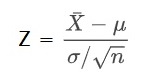
The probability is estimated by transforming the normal distribution with mean = 260 and standard deviation = 50 to a standard normal distribution (Z):

The ‘pnormGC’ function of the ‘tigerstats’ package makes it easy to depict the distribution and the region of importance.

library(tigerstats)

sample <- 20
null_mean <- 260
ssd <- 50
data <- 278.3

zz <- round((data - null_mean)/(ssd/sqrt(sample)), 2)
pnormGC(zz, region="above", mean=0, sd=1, graph=TRUE)

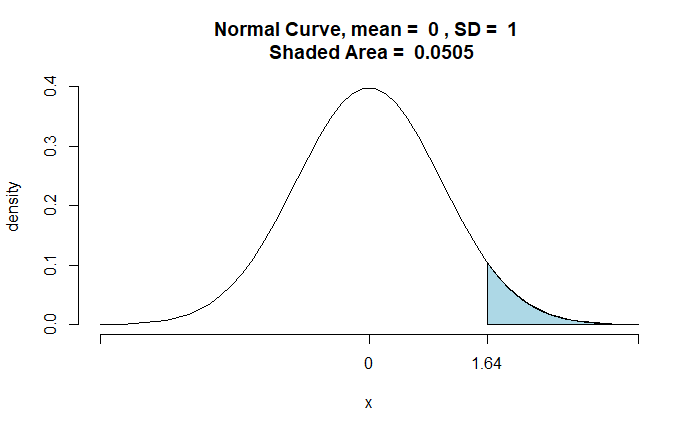
The probability of incorrectly rejecting the null hypothesis is 0.0505 (5.05%). It is the probability of Alan committing a Type I error.

If Alan accepts a 5% Type I error, he will reject the null hypothesis for every value > 278.3 and accept all values < 278.3.

2. If so, what is the probability of wrongly rejecting the alternate hypothesis that the true population mean for this year = $290?

sample <- 20
alt_mean <- 290
ssd <- 50
data <- 278.3

zz1 <- round((data - alt_mean)/(ssd/sqrt(sample)), 2)
pnormGC(zz1, region="below", mean=0, sd=1, graph=TRUE)

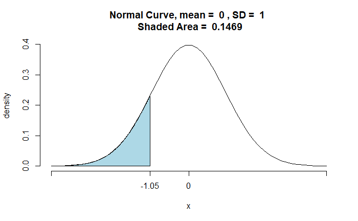
The shaded area represents all the values < 278.3. And it is the probability of Type II error.

Type I, Type II and pnormGC! Read More »

Reproducibility and Replicability

If I were to define science in one phrase, it would be ‘hypothesis testing’. In the report published in 2019, the committee appointed by the Science Foundation (NSF) defined two fundamental terms connected to scientific research (and hypothesis testing): reproducibility and replicability.

Reproducibility

Reproducibility is about computation. It is about consistent calculation output from the same input data, computational steps, methods, codes, etc.

Replicability

Replicability involves new data collection using methods similar to those employed by previous studies.

References

National Academies of Sciences, Engineering, and Medicine 2019. “Reproducibility and Replicability in Science“. Washington, DC: The National Academies Press. https://doi.org/10.17226/25303.

Reproducibility and Replicability Read More »

Three Recommendations on the p-Value Threshold

In the previous post, we saw the problem of indiscriminately using the threshold p-value of 0.05 to test significance. Benjamin and Berger, in their 2019 publication in The American Statistician, urge the scientific community to be more transparent and make three recommendations to manage such situations.

Recommendation 1: Reduce alpha from 5% to 0.5%

It is probably a pragmatic solution for people using p-value-based null hypothesis testing. We know 0.005 corresponds to a Bayes Factor of ca. 25, which can produce good posterior odds for prior odds as low as 1:10. But what happens if the prior odds are lower than 1:10 (say, 1:100 or 1:1000)?

Recommendation 2: Report Bayes Factor

Bayes factor gives a different perspective on the validity of the alternative hypothesis (finding) against the null hypothesis (default). Once it is reported, the readers will have a feel of the strength of the discovery.

Bayes Factor (BF10)Interpretation
> 100Decisive evidence for H1
10 – 100Strong evidence for H1
3.2 – 10Substantial evidence for H1
1 – 3.2No real evidence for H1

Recommendation 3: Report Prior and Posterior Odds

The best service to the community is when researchers estimate (and report) the prior odds for the discovery and how the evidence has transformed them to the posterior.

Reference

[1] Benjamin, D. J.; Berger, J. O., “Three Recommendations for Improving the Use of p-Values”, The American Statistician, 73:sup1, 186-191, DOI: 10.1080/00031305.2018.1543135

[2] Kass, R. E.; Raftery, A. E., Bayes Factors, Journal of the American Statistical Association, 1995, 90(43), 773

Three Recommendations on the p-Value Threshold Read More »

Bayes Factor and p-Value Threshold

Blind faith in p-value at 5% significance (p = 0.05) has contributed to a lack of credibility in the scientific community. It has affected the class, ‘discoveries’ more than anything else. Although the choice of threshold p-value = 0.05 was arbitrary, it has become a benchmark for studies in several fields.

It is easier to appreciate the issue once you understand the Bayes factor concept. We have established the relationship between the prior and posterior odds (of discovery) in an earlier post:
Posterior Odds = BF10 x Prior Odds

Studies show that the prior odds of typical psychological studies are 1:10 (H1 relative to H0). For clarity, H1 represents the hypothesis leading to a finding, and H0 is the null hypothesis. In such a context, a p-value, which is equivalent to a Bayes factor of ca. 3.4, makes the following transformation.

Posterior Odds = 3.4 x (1/10) = 0.34 ~ (1/3); the odds are still in favour of the null hypothesis.

On the other hand, if the threshold p is 0.005 (equivalent to a BF = 26),
Posterior Odds = 26 x (1/10) = 2.6 (2.6/1); more in favour of the discovery.

Reference

Redefine statistical significance: Nature human behaviour

Bayes Factor and p-Value Threshold Read More »

Bayes Factor and Rare Diseases

Let’s revisit Sophie and the equation of life (a.k.a. Bayes’ theorem). We know that the chance of breast cancer became about 12%, starting from a state of no symptoms and a positive test result. That too from a test that has 95% sensitivity and 90% specificity. And the secret behind this mysterious result was the low prevalence or prior probability of the disease.

P(D|TP) = P(TP|D) x P(D) /[P(TP|D) x P(D) + P(TP|!D) x P(!D)]

Here, TP represents test positive, D denotes disease and !D is no disease.

Rare disease

How do you describe a rare disease? As a simple approximation, let’s define it as an illness with a chance of 1% or lower to occur. We’ll now apply the Bayes’ rule for a few cases of P(D) (0.01, 0.005, 0.001, etc) and see how the probability updates when the test comes positive.

P(D)
Prior
P(D|TP)
Posterior
Posterior
/ Prior
(ratio)
0.010.0888.8
0.0050.0469.2
0.0010.00949.4

Can you estimate the Bayes factor for the above case?

Bayes FactorD-!D = P(TP|D) / P(TP|!D)
P(TP|D) = sensitivity = 0.95
P(TP|!D) = 1 – specificity = 1 – 0.9 = 0.1
BFD-!D = 0.95 / 0.1 = 9.5

As a heuristic, for rare diseases, the updated chance of having the disease post a positive diagnostics equals Bayes factor x prevalence.

Bayes Factor and Rare Diseases Read More »

Bayes Factor – Continued

Let’s progress further the concept of Bayes Factor (BF). In the last post, the BF was defined in favour of the null hypothesis (BF01). From now on, we focus on BF10 or the Bayes factor in favour of the alternate hypothesis.

Bayes Factor10 = P(Data|H1) / P(Data|H0)

As per Bayes theorem:
P(H1|D) = [P(D|H1) P(H1)] / P(D)
P(H0|D) = [P(D|H0) P(H0)] / P(D)
[P(H1|D) / P(H0|D)] = [P(D|H1) P(H1)] / [P(D|H0) P(H0)]
[P(H1|D) / P(H0|D)] = [P(D|H1) / [P(D|H0)] [P(H1)] / P(H0)]
Posterior Odds = BF10 x Prior Odds

This definition is significant in determining the strength of the alternate hypothesis given the experimental data or P(H1|D). Note that an experimenter is always interested in it, but the traditional hypothesis testing and p-values never helped her to know it. Let’s see how it works:

Let the prior probability for your hypothesis be 0.25 (25%), which is 1:3 prior odds (note: P(H1) + P(H0) = 1 and P(H1|D) + P(H0|D) = 1). And the BF10 is 5, which is pretty moderate evidence and is not far from a p-value of 0.05. The posterior odds become 5:3 (P(H1|D) / P(H0|D)). This corresponds to a posterior probability for the alternate hypothesis (P(H1|D)) = 5/8 = 0.625 (62.5%).

So, a Bayes Factor of 5 has improved the prior probability of the hypothesis from 25% to 62.5%.

Bayes Factor – Continued Read More »

Bayes Factor

Most of the hypothesis testing we have seen so far comes under the category of what is known as the null hypothesis significance testing (NHST). In this framework, we have two competing hypotheses:

  1. The Null Hypothesis, H0, where there is no impact of an intervention
  2. Alternate Hypothesis, HA, where there is an impact of the intervention.

Hypothesis testing aims to collect data (evidence) and assess the fit for one of the above models. At the end of NHST, you either ‘reject’ or ‘fail to reject’ your Null hypothesis – at a specified significance value – using the well-known p-value.

p-value ~ P(Data|H0)

On the contrary, we can define a ratio that gives equal weightage for the null and the alternative hypotheses. That is the Bayes Factor. It compares the probability of the data under one hypothesis with the probability under the other.

Bayes Factor01 = P(Data|H0) / P(Data|H1)

If BF01 > 1, the data is likely supporting H0
If BF01 < 1, the data is likely supporting H1

Bayes Factor Read More »

Friedman test

Let’s work out another non-parametric hypothesis test – analogous to repeated measures ANOVA, the Friedman test. The way it works is exemplified by analysing ten runners who participated in a training program. The following are the measured heart rates at regular intervals. Your task is to inspect if there is a significant difference in the heart rate of patients across the three time points.

H_Rate <-  matrix(c(150, 143, 142,
                  140, 143, 140,
                  160, 158, 165,
                  145, 140, 138,
                  138, 130, 128,
                  122, 120, 125,
                  132, 131, 128,
                  152, 155, 150,
                  145, 140, 140,
                  140, 137, 135),
                nrow = 10,
                byrow = TRUE,
                dimnames = list(1:10, c("INITIAL", "ONE WEEK", "TWO WEEKS")))
INITIAL ONE WEEK TWO WEEKS
1      150      143       142
2      140      143       140
3      160      158       165
4      145      140       138
5      138      130       128
6      122      120       125
7      132      131       128
8      152      155       150
9      145      140       140
10     140      137       135

The null hypothesis, H0: HR1 = HR2 = HR3 (mean heart rates across the intervals are all equal)
The alternative hypothesis, HA: There is a difference (at least one) during the interval.

The following command can execute the Friedman test,

friedman.test(H_Rate)
	Friedman rank sum test

data:  H_Rate
Friedman chi-squared = 5.8421, df = 2, p-value = 0.05388

The p-value is 0.053, which is greater than the significance value of 0.05; the evidence is not sufficient to reject the null hypothesis.

Friedman test Read More »

Non-Parametric ANOVA – Kruskal–Wallis test

Here are five months of quality data on Ozone concentration. The task is to test if one month’s data is significantly different from any other month’s.

The first thing to graph the monthly variations of ozone in summary plots: a boxplot is one good choice.

library(ggpubr)
data("airquality")
AQ_data <- airquality
ggboxplot(AQ_data, x = "Month", y = "Ozone", 
          color = "Month", palette = c("#00AFBB", "#E7B800", "#a0AF00", "#17B800", "#20AFBB"),
        ylab = "Ozone", xlab = "Month") +
theme(legend.position="none")

Getting quantitative

Let’s do a hypothesis test. A few quick Shapiro tests suggest only month 7 followed a normal distribution. So, we will use a non-parametric test. The Kruskal–Wallis test is one of them.

kruskal.test(Ozone ~ Month, data = airquality)
	Kruskal-Wallis rank sum test

data:  Ozone by Month
Kruskal-Wallis chi-squared = 29.267, df = 4, p-value = 6.901e-06

Yes, monthly behaviours are not similar. If you want pair-wise testing, we can use a pair-wise Wilcoxon rank-sum test.

pairwise.wilcox.test(AQ_data$Ozone, AQ_data$Month)
	Pairwise comparisons using Wilcoxon rank sum test with continuity correction 

data:  AQ_data$Ozone and AQ_data$Month 

  5      6      7      8     
6 0.5775 -      -      -     
7 0.0003 0.0848 -      -     
8 0.0011 0.1295 1.0000 -     
9 0.4744 1.0000 0.0060 0.0227

P value adjustment method: holm 

The conclusion: Significant differences are seen:
Month 5 vs Month 7 and Month 8
Month 9 vs Month 7 and Month 8

Non-Parametric ANOVA – Kruskal–Wallis test Read More »