So, do you think the machine learning algorithm developed in the previous post is useful for predicting the sex of a person their height? In other words, what is the precision of the method?
The precision means the probability of the person being a female, given the prediction was for a female.
Based on Bayes’ theorem
Note that P(Y = 1) is the prior probability of females in the system and not in the dataset. It is likely to be close to 0.5. Whereas we know the prevalence of females in the dataset is 0.23 (P( Y^ = 1)). This implies the ratio, actual vs the dataset, is 0.23/0.5 = 0.46; precision is less than 1 in 2.
Confusion Matrix and Statistics

          Reference
Prediction Female Male
    Female     55   24
    Male       64  383

               Accuracy : 0.8327
                 95% CI : (0.798, 0.8636)
    No Information Rate : 0.7738
    P-Value [Acc > NIR] : 0.0005217

                  Kappa : 0.4576

 Mcnemar's Test P-Value : 3.219e-05

            Sensitivity : 0.4622
            Specificity : 0.9410
         Pos Pred Value : 0.6962
         Neg Pred Value : 0.8568
             Prevalence : 0.2262
         Detection Rate : 0.1046
   Detection Prevalence : 0.1502
      Balanced Accuracy : 0.7016

       'Positive' Class : Female
We see the prediction we did had high overall accuracy. At the same time, we see it had a low sensitivity. It happened because of the low prevalence (proportion of females), 23%. That means failing to call actual females as females (low sensitivity) does not lower the accuracy as much as it would have by incorrectly calling males as females.
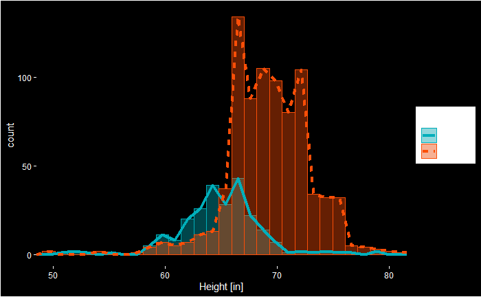
Looking at the plot, we see that the cut-off we used, 64 inches, misses a significant proportion of females. Let’s re-run the simulations after adding two more points (66 inches) to the cut-off.
Confusion Matrix and Statistics

          Reference
Prediction Female Male
    Female     82   66
    Male       33  345

               Accuracy : 0.8118
                 95% CI : (0.7757, 0.8443)
    No Information Rate : 0.7814
    P-Value [Acc > NIR] : 0.049151

                  Kappa : 0.5007

 Mcnemar's Test P-Value : 0.001299

            Sensitivity : 0.7130
            Specificity : 0.8394
         Pos Pred Value : 0.5541
         Neg Pred Value : 0.9127
             Prevalence : 0.2186
         Detection Rate : 0.1559
   Detection Prevalence : 0.2814
      Balanced Accuracy : 0.7762

       'Positive' Class : Female
Machine learning is a technique to train a model (algorithm) using a dataset for which we know the outcome and then use the algorithm, making predictions where we don’t have the outcome. The confusion matrix is the summary in a tabular form, highlighting the model performance.
Height data
We develop a simple machine learning algorithm predicting the sex of a person from the height data. The R package to help here is ‘caret’. Here are the first ten entries of the dataset that contains 1050 members.
The first thing is to check whether we can distinguish between the heights of males and females. The following command summarises the mean and standard deviation of heights.
Yes, the males are a little taller than the females, and we use this property to make decisions. I.e., assign the output as male if the height is greater than 64 inches and female otherwise. But before getting into the calculations, we divide the dataset randomly into two halves – training set and test set – using the ‘createDataPartition’ in the ‘caret’ package.
test_index <- createDataPartition(heights$height, times = 1, p = 0.5, list = FALSE)
train_set <- heights[-test_index,]
test_set <- heights[test_index,]
Now, we have two sets with 526 members each. We apply the algorithm to the training set and see the results.
Confusion Matrix and Statistics

          Reference
Prediction Female Male
    Female     55   24
    Male       64  383

               Accuracy : 0.8327
                 95% CI : (0.798, 0.8636)
    No Information Rate : 0.7738
    P-Value [Acc > NIR] : 0.0005217

                  Kappa : 0.4576

 Mcnemar's Test P-Value : 3.219e-05

            Sensitivity : 0.4622
            Specificity : 0.9410
         Pos Pred Value : 0.6962
         Neg Pred Value : 0.8568
             Prevalence : 0.2262
         Detection Rate : 0.1046
   Detection Prevalence : 0.1502
      Balanced Accuracy : 0.7016

       'Positive' Class : Female
In the tabular form,
Actual
Female
Male
Predicted
Female
55
24
Male
64
383
The rows on the confusion matrix present what the algorithm predicted, and the columns correspond to the known truth. The output provides a bunch of other metrics. That is next.
Here is the data on alcohol consumption before and after the breakup. There is an assumption that the drinking habit increases post-breakup. Is that true?
Before
After
470
408
354
439
496
321
351
437
349
335
449
344
378
318
359
492
469
531
329
417
389
358
497
391
493
398
268
394
445
508
287
399
338
345
271
341
412
326
335
467
The null hypothesis, H0: (consumption after – before) = 0. The alternative hypothesis, HA: (consumption after – before) > 0.
T-Test
D = Mean difference of the parameter after and before mud = hypothesised mean difference Sd = Standard deviation of the difference n = number of samples
We insert the data in the following command and run the function, t.test.
	Paired t-test

data:  Before and After
t = -0.53754, df = 19, p-value = 0.7014
alternative hypothesis: true mean difference is greater than 0
95 percent confidence interval:
 -48.49262       Inf
sample estimates:
mean difference
          -11.5
There was a difference of -11.5, yet the p-value (0.7014) is higher than the critical value we chose (0.05). The test shows no evidence supporting the hypothesis.
A placebo is used in clinical trials as a control in drug studies to test the effectiveness of treatments. In drug trials, one group of participants receives the medicines (to be tested), and the other gets the placebo (say, sugar pills).
The concept of placebo stems from the assumption that a treatment has two components, one related to the specific effects of the treatment and the other, nonspecific, related to its perception. When the nonspecific effects are beneficial to the participant, it is called a placebo, and when they are harmful, it is a nocebo.
Hypothesis Testing
The null hypothesis (H0) typically represents the default state or the state of “no effect“. For example, you compare the means of two groups, such as people who took a particular drug and people who received the placebo. As a drug researcher, your objective is to find the effectiveness of the medicine. And that lays the foundation for your alternative hypothesis (HA or H1) – that the drug has a non-zero effect. The default state (H0) assumes the drug has no impact. To be specific, H0 assumes the difference between two means equals zero.
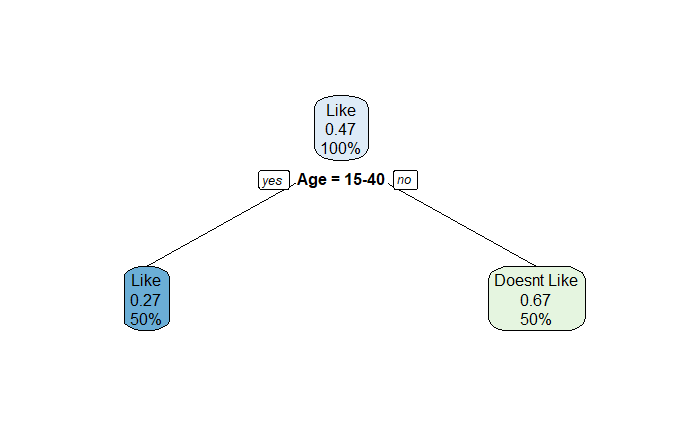
Decision trees are logical pathways created by tracing answers to multiple stages of true/false, no-go/no-go questions. Here is a representation of a simple tree based on a person liking something given their age.
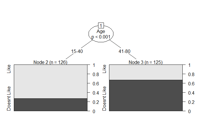
Another to represent the same info is:
A regression tree is a type of decision tree. In the regression tree, each leaf represents a numeric value. The other type is a classification tree with true/false or another category in its leaves.
The power of a statistical test is the probability of rejecting the null hypothesis when the null hypothesis is false (or the effect is present). It is the right decision, and before we go deeper into it, let’s recap the two types of errors in hypothesis testing.
A type I error is when the Null hypothesis is true, but you rejected it.
A type II error is when you fail to reject a false Null hypothesis; in other words, the effect is present.
Amelie has developed a new drug against the flu and wanted to test its effectiveness. She recruited 50 people and divided them into two groups. She gave the medicine to the first group (34 people) and provided a placebo to the second (16). Here are the results.
In the treatment group, 15 out of 34 (44%) recovered in 1 day. In the control group, 4 out of 16 (25%) recovered in 1 day.
Amelie thinks her medicine is effective because of the big defence (44 – 25 = 19%) in performance and the larger sample size for the treatment group. Do you agree?
We must do a statistical test to conclude. The data is:
Sample
Events
Trials
Treatment
15
34
Control
4
16
The Null Hypothesis, H0: No impact of medicine; recovery proportion on drug equals that of placebo. The Alternative Hypothesis, H1: Medicine improves the condition; recovery proportion on drug greater than placebo.
We use the ‘prop.test()’ function in R.
prop.test(x = c(15, 4), n = c(34, 16), alternative = "greater")
We used the one-tailed test to determine whether the treatment has improved the condition compared to the control.
	2-sample test for equality of proportions with continuity correction

data:  c(15, 4) out of c(34, 16)
X-squared = 0.97389, df = 1, p-value = 0.1619
alternative hypothesis: greater
95 percent confidence interval:
 -0.0813273  1.0000000
sample estimates:
   prop 1    prop 2
0.4411765 0.2500000
The p-value of 0.1619 (more than the significance value of 0.05) is not enough to reject the null hypothesis.
What would have happened if she had recruited more people in the placebo group and found results at the same proportions?
Sample
Events
Trials
Treatment
15
34
Control
16
64
prop.test(x = c(15, 16), n = c(34, 64), alternative = "greater")
	2-sample test for equality of proportions with continuity correction

data:  c(15, 16) out of c(34, 64)
X-squared = 2.9205, df = 1, p-value = 0.04373
alternative hypothesis: greater
95 percent confidence interval:
 0.002691967 1.000000000
sample estimates:
   prop 1    prop 2
0.4411765 0.2500000
Here, the results are significant (p-value = 0.04373 < 0.05) to reject the null hypothesis in favour of the alternate (that the drug works).
What about recruiting more to the treatment group?
Sample
Events
Trials
Treatment
150
340
Control
4
16
prop.test(x = c(150, 4), n = c(340, 16), alternative = "greater")
	2-sample test for equality of proportions with continuity correction

data:  c(150, 4) out of c(340, 16)
X-squared = 1.5631, df = 1, p-value = 0.1056
alternative hypothesis: greater
95 percent confidence interval:
 -0.02503096  1.00000000
sample estimates:
   prop 1    prop 2
0.4411765 0.2500000
p-value = 0.1056; the null hypothesis stays!
Or, had many individuals in both groups?
Sample
Events
Trials
Treatment
150
340
Control
40
160
prop.test(x = c(150, 40), n = c(340, 160), alternative = "greater")
	2-sample test for equality of proportions with continuity correction

data:  c(150, 40) out of c(340, 160)
X-squared = 16.076, df = 1, p-value = 3.042e-05
alternative hypothesis: greater
95 percent confidence interval:
 0.1149402 1.0000000
sample estimates:
   prop 1    prop 2
0.4411765 0.2500000
Both the groups have plenty of samples, and now the difference (44 – 25 = 22%) overwhelmingly supports the impact of the medicine.