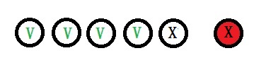
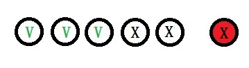
Amy and Becky are playing a game. Six cards – numbered 1 through 6 – are placed face down on the table. The cards are shuffled, and each one takes a card at random. The person with the higher number wins. Amy looks at her card and finds it is #2. Becky looks at hers and asks if Amy wants to trade her card. What should Amy’s response be? Note both players are rational.
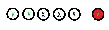
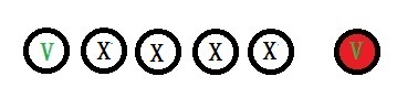
If Becky had a 6, she wouldn’t ask for a trade, as #6 is guaranteed to win. If she had #5, the only card she benefits from is #6, something Amy would never trade. That eliminates #5 and #6 from the game. By extending the logic, 4 and 3 are also eliminated. That leaves #1 something Becky is happy to offer, but Amy will never accept.
So Amy’s answer to the call is a NO.
These types of games are known as the Iterated Elimination of Strictly Dominated Strategies (IESDS).
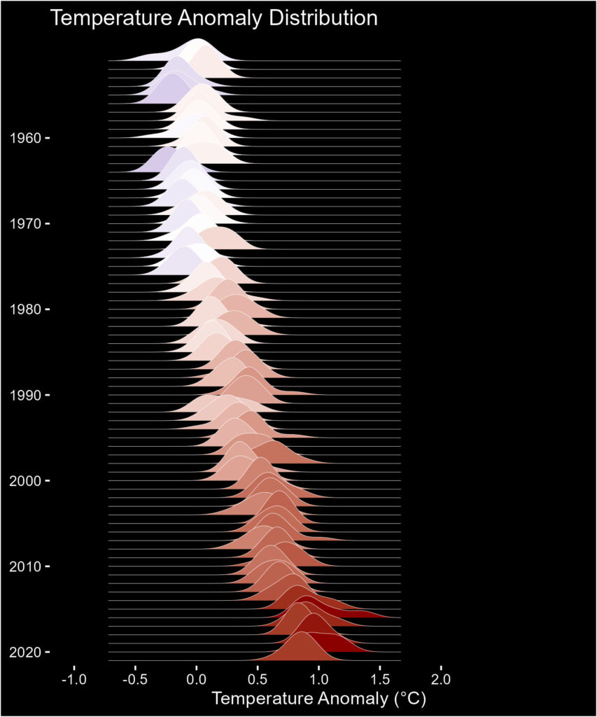
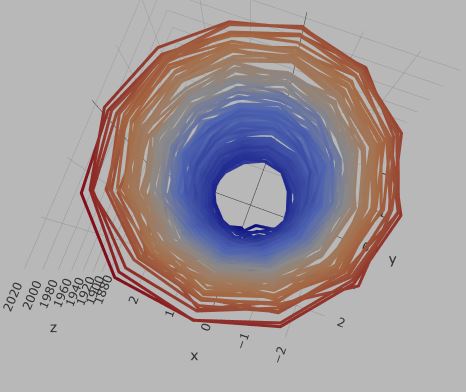
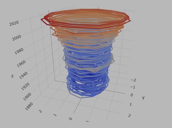
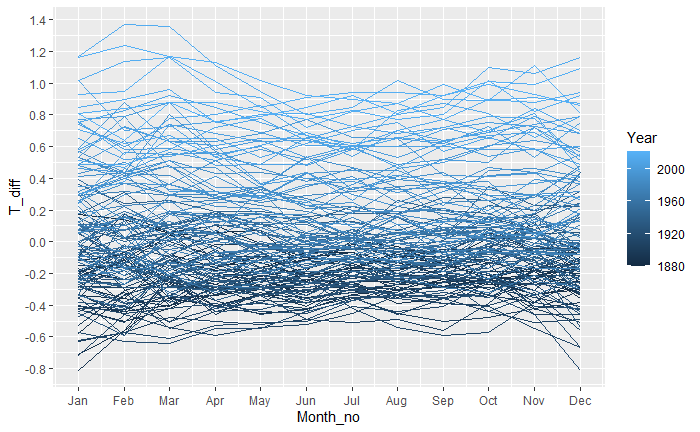
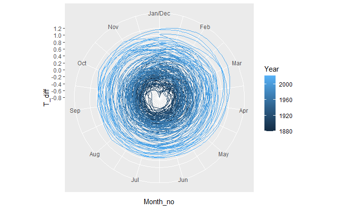
In the last post, we initiated the plotting of the abnormal temperature differences over the years (from the standardised values) thought to have been arising out of global warming. Today, we will build the famous spiral plot to visualise it.
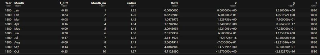
First, we transform the data to polar coordinates.
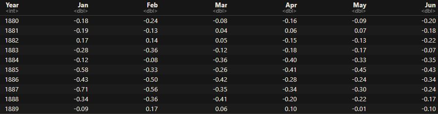
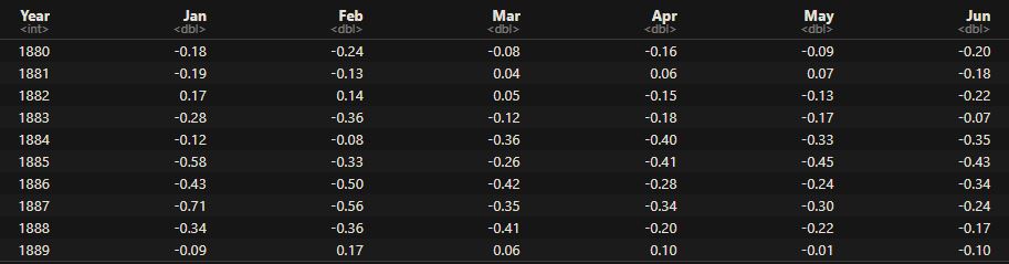
Let’s construct a visualisation of global temperature change – from 1880 – similar to what the British climate scientist Ed Hawkins did. The data used in the exercise has been downloaded from the GitHub channel of Riffomonas. He tabulated the deviation in the annual global mean from the data normalized between the temperatures 1951 – 1980.
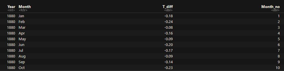
The first step is to pivot the data into the following format:
As per CDC, male condoms as a contraceptive has a failure rate of 13% for typical use and 3% for perfect use. The question is: what does it mean? The website doesn’t clarify further.
Possibility 1: a woman will get 13% of the times she has sex using a condom.
If that is true, using the protection once a month (during fertile days), a binomial equation tells you there is an 81% chance of getting pregnant in a year; (1 – (1-0.13)12)*100 = 81. It is no different from the approximate chances of conception for a woman without fertility issues.
The correct interpretation of the statistic is that it’s the number of pregnancies when 100 women use that birth control method for one year. Putting the number 0.13 back in the binomial equation, one can get the condom failure probability of about a per cent. That is pretty impressive.
Three bags, each containing ten balls, with the following combinations: 1) 3 red, 7 black 2) 8 red, 2 black 3) 4 red, 6 black One of the bags is randomly selected, and a ball is drawn. If the ball drawn is red, what is the probability that it is taken from the third bag?
A player rolls a die and can win the number of dollars equal to the number on the die except when the die shows a 6. If a 6 is rolled, the player loses $6. If the game is to be fair, what should be the cost to play?
So, what is a fair game? A fair game is something where the expected value is zero. Let’s plug in all the numbers and the unknown (the cost) in the expected value calculations.
E = (1 + 2 + 3 + 4 + 5)/6 – 6/6 = 9/6 = 1.5
The expected value is $1.5. So the game can charge $1.5 to make it fair.
We have estimated the expected value of the Powerball to be about -$1.54, but for a base prize for a jackpot of $20 mln. The money will roll over to the next if there’s no winner. So there is a probability of increasing the prize to higher and higher.
So, how can one increase the expected value? EV is a product of two parameters, but one can not modify the ‘probability’, which is fixed as in the combination calculation we did earlier. As mentioned earlier, the jackpot amount grows in case there are no winners, implying an increase in the expected value.
It is good news and bad news. The good news is that the number of tickets sold increases as the prize gets heavier and the chance of winning (as per the binomial distribution). The bad news is the number of winners who will eventually share the jackpot also increases.
I see recommendations to choose unique numbers to reduce the chance of sharing, but that looks silly. The person, shared or not (plus taxes), is more likely to get more than the $2 she spent on the ticket as the jackpot! So why waste time selecting what she thinks is unique?
So, there is a 95.98% chance that you win nothing, and the expected value of the affair is -$1.54. To remind you, the expected value is the money I can make in the long run.
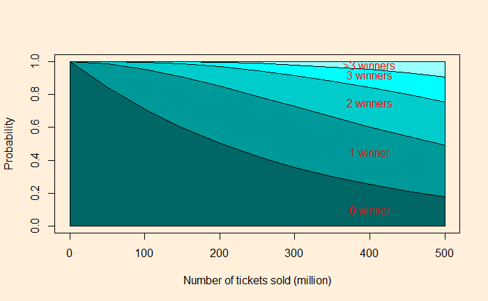
Not to forget, if the number of tickets sold increases, there could also be multiple people winning it, splitting the prize. Here is the probability of winning the jackpot estimated using the binomial distribution.
Here is the R code of the above plot:
xx <-   seq(0, 500, 50)
yy <-   dbinom(x = 0, size = xx, prob = 1/292.201338)
yy1 <-  dbinom(x = 1, size = xx, prob = 1/292.201338)
yy2 <-  dbinom(x = 2, size = xx, prob = 1/292.201338)
yy3 <-  dbinom(x = 3, size = xx, prob = 1/292.201338)
yy4 <-  1 - pbinom(3, size = xx, prob = 1/292.201338)

par(bg = "antiquewhite1")
plot(xx,yy, ylim = c(0,1), type ="l", col = "red", xlab = "Number of tickets sold (million)", ylab="Probability")
polygon(x = c(0, xx, 500), y = c(0, yy, 0), col = "#006666")
text(x = 400, y = 0.1, "0 winner", col = "red")
lines(xx,yy+yy1, col ="blue" )
polygon(c(xx, rev(xx)), c(yy+yy1, rev(yy)),col = "#009999")
text(x = 400, y = 0.45, "1 winner", col = "red")
lines(xx,yy+yy1+yy2, col = "green" )
polygon(c(xx, rev(xx)), c(yy+yy1+yy2, rev(yy+yy1)), col = "#00cccc")
text(x = 400, y = 0.75, "2 winners", col = "red")
lines(xx,yy+yy1+yy2+yy3, col = "brown" )
polygon(c(xx, rev(xx)), c(yy+yy1+yy2+yy3, rev(yy+yy1+yy2)), col = "#00ffff")
text(x = 400, y = 0.92, "3 winners", col = "red")
lines(xx,yy+yy1+yy2+yy3+yy4, col = "black" )
polygon(c(xx, rev(xx)), c(yy+yy1+yy2+yy3+yy4, rev(yy+yy1+yy2+yy3)), col = "#99ffff")
text(x = 400, y = 0.98, ">3 winners", col = "red")
So, there is a 1/292201338 chance of winning a jackpot at the Powerball. That means if the prize is $20 million, the expected value of a ticket is $20,000,000 x 1/292201338 = $0.068. Not to forget, it includes the value to the individual and the state, which takes over half of the winning amount as taxes!
Consolation prizes
The jackpot is not the only thing you get; there are a few more things you win, as follows.
Match
Prize
Five whites
$1,000,000
Four whites + red
$50,000
Four whites
$100
Three whites + red
$100
Three whites
$7
Two whites + red
$7
One white + red
$4
Red
$4
Let’s look at the probabilities next.
Five whites and no red
P(5W AND NR) = P(5W)xP(NR) P(5W) = 1 / 69C5 = 1/11238513 P(NR) = (25/26) P(5W AND NR) = (1/11238513) x (25/26) E.V. (5W AND NR) = $1,000,000 x 25 / (11238513 x 26) = $0.085
Four whites and One red
P(4W AND 1R) = P(4W)xP(1R) P(4W) = How many ways of getting 4 winning numbers of 5 drawn out of all combinations of 5 from 69 = How many ways of getting 4 winning numbers of 5 drawn x How many ways of the remaining 1 is not / How many ways of getting 5 winning numbers of 5 drawn from 69 = (5C4 x 64C1) / 69C5 = 320 / 11238513 P(1R) = (1/26) P(4W AND 1R) = (320/11238513) x (1/26) E.V. (4W AND 1R) = $50,000 x (320/11238513) x (1/26) = $0.055
Four whites and no red
P(4W AND NR) = P(4W)xP(NR) P(4W AND NR) = (320/11238513) x (25/26) E.V. (4W AND NR) = $100 x (320/11238513) x (25/26) = $0.0027
Three whites and One red
P(3W AND 1R) = P(3W)xP(1R) P(3W) = (5C3 x 64C2) / 69C5 = 20160/ 11238513 P(1R) = (1/26) P(3W AND 1R) = (20160/11238513) x (1/26) E.V. (3W AND 1R) = $100 x (20160/11238513) x (1/26) = $0.007
Three whites and no red
P(3W AND NR) = P(3W)xP(NR) P(3W AND NR) = (20160/11238513) x (25/26) E.V. (3W AND NR) = $7 x (20160/11238513) x (25/26) = $0.012
Two whites and One red
P(2W AND 1R) = P(2W)xP(1R) P(2W) = (5C2 x 64C3) / 69C5 = 416640/ 11238513 P(1R) = (1/26) P(2W AND 1R) = (416640/11238513) x (1/26) E.V. (2W AND 1R) = $7 x (416640/11238513) x (1/26) = $0.01
One white and one red
P(1W AND 1R) = P(1W)xP(1R) P(1W) = (5C1 x 64C4) / 69C5 =3176880/ 11238513 P(1R) = (1/26) P(1W AND 1R) = (3176880/11238513) x (1/26) E.V. (1W AND 1R) = $4 x (3176880/11238513) x (1/26) = $0.04
Zero whites and One red
P(0W AND 1R) = P(0W)xP(1R) P(0W) = (64C5) / 69C5 = 7624512/ 11238513 P(1R) = (1/26) P(0W AND 1R) = (7624512/11238513) x (1/26) E.V. (0W AND 1R) = $4 x (7624512/11238513) x (1/26) = $0.1
The Math of Powerball: Think Big The odds you’ll win the Powerball jackpot: CNBC