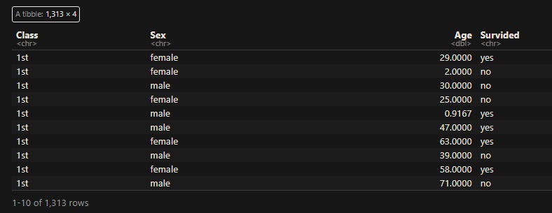
Data & Statistics

Powerball

In the Powerball drawing, the numbers are selected from two containers. Five white balls from 69 balls numbered 1 through 69 and one from 26 balls (1-26). To win the Powerball jackpot, the person must watch all six balls. What is the probability of winning the jackpot if you buy a Powerball ticket?

The probability of winning the jackpot = the probability of winning five numbers from the first pot x the probability of winning the number from the second pot. And the good news is, the order doesn’t matter. So you have one way of getting out of the so many ways of drawing five white balls. And since the order doesn’t matter, as you know, it is a combination problem.

So you have one chance out of 69C5 ways of getting five white balls AND 26 ways of getting the red ball. Or 1/(69C5 x 26) = 1/292201338. In case you forgot, the formula for combination, s balls from n possibilities,

The number of combinations of n things, taken s at a time = [n!/s!(n-s)!]

Finally, is it worth spending $2 for a ticket that offers a jackpot of $20 million? We’ll see next.

Powerball Read More »

Scope Neglect 

Scope neglect is a cognitive bias in which a person fails to comprehend the difference in the magnitude of numbers. A simple example is the difference between 1 billion and 1 trillion. Most people know a trillion is different, but it is difficult to imagine it is 1000 times bigger than a billion.

Scope neglect or insensitivity occurs because we are unable to visualise large numbers. When one can’t picture large numbers, they remain in abstract form, failing to create the expected level of emotional reaction.

In one study, the participants were asked what they would contribute to saving 2000, 20000 or 200,000 birds from drowning in oil-contaminated ponds. The answers were $80, $78 and $88, respectively!

Scope Neglect  Read More »

The Sailor’s Child problem

A sailor sails between two ports. At each port, he stays with a woman, both of whom want to have a child with him. The sailor is initially reluctant but changes his mind and tosses a coin to decide: if it’s a head, he will have a child with one and if it’s tail, with both. If heads come up, he will open up The Sailor’s Guide to Ports, and whichever port, out of the two, features earlier, he will choose the woman on that port.

If A is the son of the sailor, what is the probability that he is an only son?

We’ll go to the Bayes’ to find out the answer.

\\ P(O|C) = \frac{P(C|O) * P(O)}{P(C|O) * P(O) + P(C|NO) * P(NO)} \\ \\ P(O|C) = \frac{(1/2) * (1/2)}{(1/2) * (1/2) + 1 *(1/2)} = \frac{1}{3}

The Sailor’s Child problem Read More »

The Heat of the Momentum

Yesterday night (or earlier today, for some), the Miami Heat beat Boston Celtics to win the Eastern Conference final of the NBA, thus qualifying for the ultimate showdown against the Denver Nuggets. The Heat made it in the seventh game after both teams had tied at 3-3.

In many ways, the matchup has been a nightmare that threw sports analysts and Las Vegas for a complete spin. For those who missed the plot, Celtics were the pre-series favourites but lost the first three matches to the Heat. The Heat obtained the momentum to make the fourth win for a sweep but lost the next three games and gave the momentum back to the Celtics. And the Celtics, not knowing that they have this thing called momentum, lost cheaply against the Heat.

The momentum of sports

Momentum is a term borrowed from physics, defined as the product of mass and velocity, a parameter with magnitude and direction. Journalists use it to represent some internal force of nature (psychology) that moves entities (sports teams, stock prices) to one direction based on their immediate past performances.

Momentum, like a hot hand, positive energy and negative energy, is a type of cognitive illusion. An argument that is often used to explain a complex or a random process. While hot hands may be partially explainable as it happens due to someone’s mood or a form on a day, this momentum thing happens over a few days. The three-match stretch may appear to you like a sequence, but each game breaks for 45 hours before the next one; most professional teams recover from such setbacks. And every game becomes a new matchup, unconnected to the previous; like a coin toss.

One can argue it was a reverse momentum that happened in this series. The fourth match became the must-win for the Celtics. And as it happened several times in the past two years, they successfully dragged themselves out of the hole, not once, but three times. Then it became a must-win for the Heat (well, also for the Celtics), which they successfully executed.

The Heat of the Momentum Read More »

Advantage Dice

You play a game in which you throw two dice (6-sided) and select the highest value. Repeat it many times. What is the average of the results?

itr <- 100000
play <- replicate(itr, {
first <- sample(c(1,2,3,4,5,6), 1, replace = TRUE, prob = c(1/6,1/6,1/6,1/6,1/6,1/6))
second <- sample(c(1,2,3,4,5,6), 1, replace = TRUE, prob = c(1/6,1/6,1/6,1/6,1/6,1/6))

max(first, second)  
})

mean(play)

The answer is 4.47

What happens if you do the same game on two 20-sided dice?

itr <- 100000
play <- replicate(itr, {
first <- sample(seq(1,20), 1, replace = TRUE, prob = rep(1/20,20))
second <- sample(seq(1,20), 1, replace = TRUE, prob = rep(1/20,20))

max(first, second)  
})

mean(play)

You get 13.83

Advantage Dice Read More »

Car with No Rear View

Imagine you get a chance to buy a coffee shop. Here is what the owner tells you.
The current sales = $ 74,000 /yr
Shop rent = $30,000 /yr
Employee salary = $25,000 /yr
Coffee beans = $15,000 /yr
The cost of furniture and coffee machine = $45,000

How much are you willing to pay?

Market value

A simple valuation shows the shop can generate $4,000 a year (74,000 – 30,000 – 25,000 – 15,000) after paying for the rent, salaries and the purchase of the coffee beans. If you feel the shop will generate the same forever, you can do a simple (perpetuity) formula of 4000 / 0.1 = 40,000; 0.1 represents the discount rate of 10%. So you are willing to pay a maximum of $40,000.

The owner reminds you that she spent 45,000 just a few weeks ago to renovate. Will you change your mind? Sadly, it shouldn’t. The cost the owner sunk in the past can’t change the value it generates in the future. The buyer politely replies that she could get $500 more ($4,500) every year if she invested that 45,000 in the market at a 10% return. So what the owner spent (the book value) is immaterial to the buyer who calculated the market value.

Movie or football

Mat bought a ticket for a movie by paying $25. Just before he starts, he gets a phone call from John, who invites him to watch a football match. Mat likes football and John’s company, yet declines the invite because he has already spent the ticket price of the movie.

The money Mat spent is sunk, and what matters now is what gives him a good time (movie vs football with friends). But Mat falls for the sunk cost fallacy, the bad feeling for the loss on things that have already been spent against a better return in the future.

The concord of failures

The fallacy of sunk cost is common in big projects. Companies often hesitate to shut down projects midway when even they realise that it’s getting expensive and the product won’t make any economic benefit. They rationalise they invested too much to quit.

Social scientists hypothesise three reasons for this fallacy

  1. The loss aversion
  2. Desire not to appear wasteful
  3. To force one to do things that otherwise won’t happen

Psychology of decision making

The sunk cost fallacy is a powerful force that impacts decision-making. The issue with sunk costs is that they are the things of the past, but we pay too much attention to them. It’s the same feeling that keeps you attending the whole show of a terrible movie, eating everything ordered even when you are full, or continuing a nonfunctional relationship solely because the couple spent four years of their life together.

Reference

Sunk Costs: The Big Misconception About Most Investments: Sprouts

Car with No Rear View Read More »

Mean, Median and Bill Gates

We have seen that the two most commonly used ways of summarising the centre of variation of observed values are the mean and the median. The mean is the numerical average, and the median is the mid-point.

Andrew Vickers uses the following example to illustrate the need for two parameters and the issue when there are outliers. Seven people with annual incomes of $85,000, $50,000, $60,000, $40,000, $75,000, $100,000 and $45,000 are in a dinner. Bill Gates walks in. What is the new distribution of the salary in the room?

Before Gates

Before Mr Gates walked in, the average salary was ($85,000 + $50,000 + $60,000 + $40,000 + $75,000 + $100,000 + $45,000) / 7 = $65,000. To estimate the median, we first need to arrange the numbers in ascending order, $40,000, $45,000, $50,000, $60,000, $75,000, $85,000, $100,000, locate the midpoint, i.e., $60,000, which is the median.

After Gates

The picture changes once Mr Gates enters the room. Let’s assume his annual income (!) is $ 1 B (the highest number I could envision). The mean is = 1,000,455,000 / 8 = $ 125 million and a bit. And the median? ($60,000 + $75,000)/2 = $67,500.

You might say the median ($67,500) better represents the crowd of upper-middle-class people (and one billionaire). The mean, the so-called average, appears helpless here.

The session cannot be complete without invoking my favourite plot of all – the box plot.

You may have noticed that 7 out of 8 fall below the mean.

Reference

What is a p-value anyway? 34 Stories to Help You Actually Understand Statistics:  Andrew Vickers

Mean, Median and Bill Gates Read More »

Contingency Table and Mosaic

table(T_data$Sex, T_data$Survided)
table2 <- table(T_data$Sex, T_data$Survided)
mosaicplot(table2, main = "Titanic Data",
           sub = "",
           xlab = "Sex",
           ylab = "Survided",
           las = 1,
           color = c("skyblue2","lightgreen"),
           border = "chocolate")
table2 <- table(T_data$Sex, T_data$Survided)
fisher.test(table2)

chisq.test(table2, correct = FALSE)

Contingency Table and Mosaic Read More »

Simpson’s Paradox – Mosaic Plot

We have seen Berkeley data in the previous post and refreshed the concept of Simpson’s paradox. Here we introduce a handy visualisation of such data using mosaic plots.

The following R code generates the mosaic plot for the overall admission. The code requires the ‘vcd’ package.


mosaic( ~   Gender + Admit, data = berk_data,
       highlighting = "Gender", highlighting_fill = c("pink", "lightblue"),
       direction = c("v","h"))

The lower width of the pink panel on the admission (top) suggests a smaller number of females (89) compared to males (512). The smaller width of the top pink panel compared to the bottom pink panel indicates lower admission rates for females (proportional to the application rate). Smaller heights of pannels indicate more rejection than admission.

Once the data is stratified to include the department, the picture changes to the following.

mosaic( ~ Dept  + Gender + Admit, data  = berk_data,
       highlighting = "Gender", highlighting_fill = c("pink", "lightblue"),
       direction = c("v","v","h"))

Most of the pink panels on the top are more than or equal to the ones on the bottom, suggesting better admission rates for females. You can check the last table of the previous post and recognise that the admission rates of departments A and B are more than 50%, and the rest are lower. Lastly, the number of male applicants is much more in those two departments (width of the blue panel compared to pink).

Simpson’s Paradox – Mosaic Plot Read More »