Data & Statistics

A Vegan View of Health

The Netflix documentary, ‘What the Health’, may belong to a class of faulty reasoning known as propaganda. Let’s look at some of the logical fallacies committed by the program.

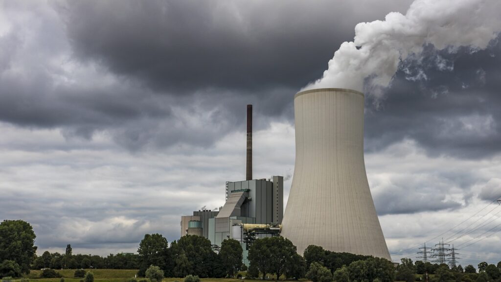
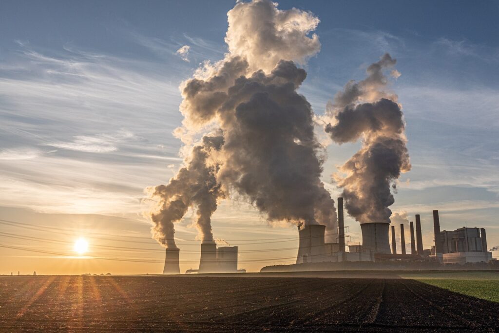
The documentary intends to promote Veganism, which, I think, is fair. Food accounts for about 25% of greenhouse gas emissions, of which meat occupies half. However, the tactics used by the producer of the film range from cherry-picking to total misinformation.

Meat and cancer

The program begins with the infamous connection between processed meat and (colorectal) cancer, which comes from the 2015 findings in the International Agency for Research on Cancer (IARC). One main suspect is the production of polycyclic aromatic hydrocarbons (PAHs) during cooking by panfrying, grilling, or barbecuing. This has led to the classification of processed meat in Group 1 (Carcinogenic to humans) and red meat in Group 2A (Probably carcinogenic to humans) as per IARC.

Statistics of the low base

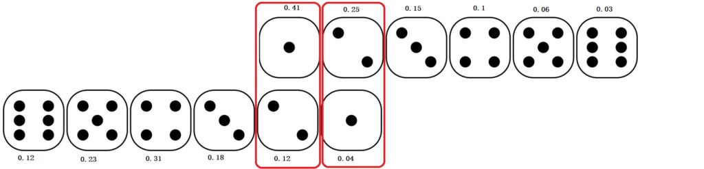
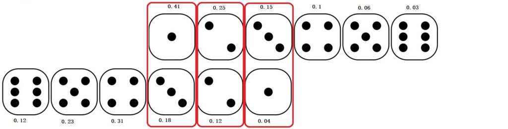
We already know the background of the study and what an 18% increase means. In simple language, the average prevalence of colorectal cancer (5 in 100) becomes 6 for meat eaters. As a comparison, smoking makes the lifetime risk of lung cancer 17.2 in 100 vs. 1.3 in 100 for non-smokers – a 1000% increase.

Appeal to fear

The program also chooses some of the fellow 126 candidates, such as Plutonium, Asbestos and cigarettes, to emphasise the seriousness of Group 1. On the other hand, it conveniently forgets that alcoholic beverages, areca nuts and solar radiation are a few other items on the same list. To reiterate, the items in one group do not have the same risk. A place in Group 1 only means the association (with cancer) is established for that item and nothing about the absolute risk.

Sugar-coated binary

The film then argues with the help of a few ‘experts’ that sugar, considered many as a problem molecule, plays no role in diseases such as diabetes. Such creation of the innocent-other to demonise the intended subject was totally unnecessary.

Missing the balances

The documentary slips into propaganda because it misses the balance. There is no debate here about the need to incorporate more plant-based diet and exercise in the lifestyle. It is also important to have the right amount of micronutrients and protein in the diet, which may include meat, egg and dairy products.

The documentary is propaganda as it primarily appeals to emotion. The objective is to form opinions rather than increase knowledge. It uses strategies such as cherry-picking, appealing to fear and misinformation.

References

IARC Report on Processed Meat

Known Carcinogens: Cancer.org

Carcinogenicity of Processed Meat: The Lancet Oncology

How common is colorectal cancer: cancer.org

Carbon Footprint Factsheet: umich

Climate change food calculator: BBC

IARC Classifications: WHO

IARC Group 1 Carcinogens: Wiki

Lung cancer by smoking: Pub Med

A Vegan View of Health Read More »

Birthday Problem – Data

We have seen the birthday problem earlier, and a group of 23 has a 50% chance that two of its members will share a birthday. Here is a real test to validate it. We use birth data from the recently concluded women’s World Cup. The data is available in the reference.

The following R code arranged the data of 736 players that belonged to 32 teams.

F_data <- read.csv("D:/Misc/DataData/Footer1.csv")
F_data <- as.data.frame(matrix(F_data$DOB, nrow = 23))
names(F_data) <- paste0("TEAM", 1:ncol(F_data))
as_tibble(F_data)

The next set of calculations modifies the dataset into a month-date format.

F_data1 <- F_data
for (i in 1:ncol(F_data)) {
  F_data1[,i] <- as.Date(F_data[,i], format = "%d/ %m/ %Y")
  F_data1[,i] <- format(F_data1[,i], format="%m-%d")
}
as_tibble(F_data1)

The final set of codes calculates if any date is duplicated in each team and gets the total number of such instances.

match1 <- rep(0, ncol(F_data1))
for (i in 1:ncol(F_data1)) {
match1[i] <- any(duplicated(F_data1[,i]) == TRUE)
}

match1
sum(match1)
0 0 1 1 0 1 1 1 0 1 1 1 0 1 0 0 1 0 0 1 1 1 0 0 0 1 0 0 0 1 1 1 

17

Since for a 23-member group, there is a 50% chance. Therefore, in a 30-team competition, the expectation is 16 teams on average. And in reality, it turned out to be 17; not bad, eh?

Reference

Squad List: women’s world cup

Birthday Problem – Data Read More »

Bayesian Snow Flakes

Alice says there was snowfall last night. Becky says Alice lies 5 out of 6 times. Carol checked the previous day’s weather prediction and said the probability of snow was 1/8. What is the probability that there was snow?

We will use Bayes’ theorem to get the answer:

P(SN|AS) – Probability that it snowed, given Alice said so.
P(AS|SN) – Probability that Alice said snowed, given there was snow.
P(SN) – Prior probability of having snow.
P(AS|NS) – Probability that Alice said snowed, given there was no snow.
P(NS) – Prior probability of having no snow.

\\ P(SN|AS) =  \frac{P(AS|SN)*P(SN)}{P(AS|SN)*P(SN) + P(AS|NS)*P(NS)} \\ \\ \frac{(1/6)(1/8)}{(1/6)(1/8) + (5/6)(7/8)} = \frac{1}{36}

1/36

Bayesian Snow Flakes Read More »

Probability of Double Dice – Convolution

We have seen how the probability of double dice can be estimated by flipping and sliding the outcomes of the second die. Here is another example to illustrate the concept: this time, with two dice with different probabilities.

0.41 x 0.04 = 0.0164

0.25 x 0.04 + 0.41 x 0.12 = 0.0592

0.15 x 0.04 + 0.25 x 0.12 + 0.41 x 0.18 = 0.1098

Why X+Y in probability is a beautiful mess: 3Blue1Brown

Probability of Double Dice – Convolution Read More »

Cooling Tower Fallacy

Can displaying wrong images justify a right cause? Today, we discuss pollution.

It is no longer a matter of debate that pollutants cause massive health hazards. As per the World Health Organisation (WHO), air pollution caused 4.2 million premature deaths worldwide in 2019. Most of it is manifested via cardiovascular and respiratory diseases and cancer.

The following are the five main entities that cause air pollution. Those are
Particulate matter (PM)
Carbon monoxide (CO)
Ozone (O3)
Nitrogen dioxide (NO2)
Sulfur dioxide (SO2)

You may have noticed the conspicuous absence of carbon dioxide in this list. This is because CO2 is not a pollutant but a greenhouse gas that causes global warming. So, it is a bad actor, though not exactly the way one would imagine.

Now, the fallacy: below is a photo I got when I typed ‘pollution’ in the image search column, followed by another picture that came up for ‘carbon dioxide’.

power plant, cooling tower, coal-fired power station-4349830.jpg
power plant, air pollution, coal-fired power station-6698838.jpg

The sorry thing is that neither of these shows pollutants nor CO2. These are images of cooling towers emitting water vapour; journalists have been using such images from power plants and other industries for ages to represent pollution and global warming. The reason? They make excellent visuals of dense plumes, captivating the readers. According to a 2007 Royal Society of Chemistry survey report, more than two-thirds of people in the UK believe these images are of carbon dioxide emissions and accelerating climate change.

Myth of cooling towers is ..: RSC

Ambient (outdoor) air pollution: WHO

Cooling Tower Fallacy Read More »

Probability of Double Dice

We have seen how the probability of getting a given sum can be estimated pictorially when two dice are thrown. It is done by displaying all possible combinations of 6 outcomes each (total of 6 x 6 = 36) and then counting the number of pairs for a given sum.

You will see these pairs along the diagonals.

For example, the probability of getting a sum of four is 3/36 by counting along the line that passes through all 4s. And if you do it for each diagonal, you get the following distribution.

There is an even smarter way to reach the above. It is done by listing the outcomes of the first die on the top row, flipping around the one from the second die and placing it below.

All the pairs that add up to seven appear as shown below. There are six of them.

Slide the second row to the right by one, and you get the 8s (5 out of 35).

This flipping (and then sliding) is a convenient way to understand convolution!

Probability of Double Dice Read More »

Accident on a Highway

If there is a 75% probability of accidents in an hour on a highway, what is the chance of accidents in 30 minutes? How many hours does it take for the highway to have an accident almost certain (i.e., 99%)?

We’ll do it in two different ways: first, the analytical.

Let p be the probability of at least one accident in 30 minutes. Then 1 – p is the chance of having no accidents in 30 minutes. Since accidents at a given moment are independent of some other moment, we can apply the AND rule, and the probability of no accidents in one hour is a joint probability of having no accidents in two consecutive half hours.
(1-p) x (1-p) = 1 – 0.75
(1-p)2 = 0.25
1 – p = 0.5
p = 0.5 = 50%

Another way to estimate these probabilities is to apply the Poisson distribution.

1 - ppois(q = 0, lambda = 1.4)
0.75

where,
q: number of successes
lambda: average rate of success

We adjusted lambda to match 0.75, which turned out to be 1.4 (accidents per hour). To get the probability for 30 minutes, use the same function for the rate of 1.4/2 accidents per half an hour.

1 - ppois(q = 0, lambda = 0.7)
0.503414

99% chance

Increase the lambda until the 1 – ppois reaches 0.99.

1 - ppois(q = 0, lambda = 4.9)
0.992

4.9 / 0.7 = 7 times 30 minutes = 3.5 hours.

Or

1- (0.5)7 = 0.99

Accident on a Highway Read More »

Chi-square – Interpretation

Un-VaccinatedVaccinated
(O-E)2/E(O-E)2/E
Contracted
pneumococcal pneumonia
5.785.78
Contracted
another type of pneumonia
0.110.11
Did not contract pneumonia0.930.93

You can see that the largest numbers for the chi-squares are against the row: ‘Contracted pneumococcal pneumonia’. These mean the largest departure from the expected values.

Un-VaccinatedVaccinated
(O-E)2/E(O-E)2/E
Contracted
pneumococcal pneumonia
(23 – 28*92/184)2/
(28*92/184)
(5 – 28*92/184)2/
(28*92/184)
Contracted
another type of pneumonia
(8 – 18*92/184)2/
(18*92/184)
(10 – 18*92/184)2/
(18*92/184)
Did not contract pneumonia(61 – 138*92/184)2/
(138*92/184)
(77 – 138*92/184)2/
(138*92/184)

In the unvaccinated case, the observation was more than the expectations (O:23 vs. E:14), whereas in the vaccinated case, it was fewer (O:5 vs. E:14).

Smaller values of chi-square suggest observed values are closer to the expected.

Reference

The Chi-square test of independence: Biochem Med 

Chi-square – Interpretation Read More »

Chi-square for Science

Science is built on the foundations of hypothesis testing. The Chi-square test of independence is one prime statistic for testing hypotheses when the variables are nominal.

The application of the Chi-square test is widely prevalent in clinical research. Here is an example of a case study published in ‘Biochemia Medica’. Following is the data from a group of 184 people, half of whom received a vaccine against pneumococcal pneumonia.

Un-VaccinatedVaccinated
Contracted
pneumococcal pneumonia
235
Contracted
another type of pneumonia
810
Did not contract pneumonia6177

1. Marginals

The first step in the Chi-square test is the calculation of the ‘marginals’. As marginals mean ‘on the sides’, we write them on the right column (the row-sums) and the bottom row (the column-sums).

Un-VaccinatedVaccinatedRow Sum
Contracted
pneumococcal pneumonia
23528
Contracted
another type of pneumonia
81018
Did not contract pneumonia6177138
Column Sum9292N = 184

2. Expected values

The chi-square test requires observed and expected values. It applies the following formula to each element and adds them up.

(O-E)2/E

The observed values are the data, and expectations are to be estimated based on the marginals. The expected data for a perfectly independent scenario is calculated as below. The expected value at (row i, column j) is obtained by RowSum(i) x ColumnSum(j)/(N).

Un-VaccinatedVaccinated
(O-E)2/E(O-E)2/E
Contracted
pneumococcal pneumonia
(23 – 28*92/184)2/
(28*92/184)
(5 – 28*92/184)2/
(28*92/184)
Contracted
another type of pneumonia
(8 – 18*92/184)2/
(18*92/184)
(10 – 18*92/184)2/
(18*92/184)
Did not contract pneumonia(61 – 138*92/184)2/
(138*92/184)
(77 – 138*92/184)2/
(138*92/184)

3. Test for Independence

Un-VaccinatedVaccinated
(O-E)2/E(O-E)2/E
Contracted
pneumococcal pneumonia
5.785.78
Contracted
another type of pneumonia
0.110.11
Did not contract pneumonia0.930.93

The Chi-square is calculated as the overall sum = 13.649

The p-value is estimated by looking at the Chi-square table for 13.349 at degrees of freedom (df) = 2.

The R code for the whole exercise

edu_data <- matrix(c(23, 5, 8, 10, 61, 77), ncol = 2 , byrow = TRUE)
colnames(edu_data) <- c("Vac", "No-Vac")
rownames(edu_data) <- c("npneumococcal pneumonia", "non-pneumococcal pneumonia", "Stayed healthy")


chisq.test(edu_data)
edu_data
	Pearson's Chi-squared test

data:  edu_data
X-squared = 13.649, df = 2, p-value = 0.001087

                           Vac No-Vac
npneumococcal pneumonia     23      5
non-pneumococcal pneumonia   8     10
Stayed healthy              61     77

The p-value suggests that the impact of vaccination on protecting against pneumococcal pneumonia is significant. And there is only a 1.1 in a thousand possibility that the difference is out of pure chance.

Reference

The Chi-square test of independence: Biochem Med 

Chi-square for Science Read More »

Picking Candies

A jar contains 60 candies, 10 reds, 20 blues and 30 yellows. If one takes out candies one by one, what is the probability that there is at least one yellow and one blue left after all the red candies have been taken out?

The solution is a combination of two mutually exclusive probabilities.

1) Probability that yellow is the 60th candy and blue is the last candy among the bunch of 10 reds and 20 blues.
OR
2) Probability that blue is the 60th candy and yellow is the last candy among the bunch of 10 reds and 30 yellows.

1a. The Probability that one of the 30 yellows is the last candy among 60 candies = 30/60
1b. The Probability that one of the 20 blues is the last candy among 30 candies = 20/30
2a. The Probability that one of the 20 blues is the last candy among 60 candies = 20/60
2b. The Probability that one of the 30 yellows is the last candy among 40 candies = 30/40

The first probability is a joint probability (‘AND’ rule) of 1a and 1b
The second probability is a joint probability of 2a and 2b
The final probability is the sum (‘OR’ rule) of the two.

(30/60) x (20/30) + (20/60) x (30/40) = 0.58

Picking Candies Read More »