Here is a game. If you win the game, you get a dollar; else, you lose one. What is the probability of winning the game?
The game involves a fair coin and two urns. Urn 1: 3 red balls; 1 blue ball. Urn 2: 1 red ball; 3 blue balls. You toss the coin first. If heads, you draw a ball from urn 1 and if tails, urn 2. Drawing a red ball wins the game.
The marginal probability of getting a head is 1/2, and getting a red ball from Urn 1 = 3/4. Therefore, the joint probability of getting a red ball from Urn 1 is (1/2)x(3/4) = (3/8). Similarly, the joint probability of getting a red ball from Urn 2 is (1/2)x(1/4) = (1/8). The overall probability of drawing a red is
(3/8) + (1/8) = (4/8) = (1/2), same as flipping a coin.
A company has bought three software packages for their operations. They are Abacus, Biscuit and Circuit. On average, Abacus crashes 1 in 200 times, Biscuit 1 in 10 times, and Circuit 1 in 50. Of the ten employees, two were assigned Abacus, five got Biscuit, and three received Circuit. If Sophia’s trial crashed on the first trial, what is the probability that she got Abacus?
If a 1-dimensional random walk starts at 0, with steps of one (to the right or left), what is the probability of reaching -30 before reaching 10?
Suppose P30 is the probability of reaching -30, and (1−P30) is the probability that to end with 10.
Let X be the position on the x-axis at the end of this game E[X] = -30 x P30 + 10 x (1-P30) For a random walk with equal steps (+1 or -1), E[X] = 0. 0 = -30 x P30 + 10 x (1-P30) -10 = P30(-30 -10) P30 = 1/4 = 0.25 = 25%
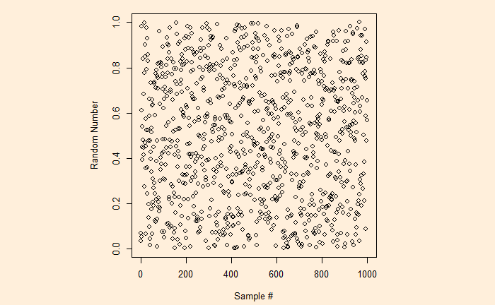
We know the ‘sample’ function creates a random sample of elements from a vector. But if you want to get a random sample between two limits, ‘runif’ is the function. Here is a plot of 1000 samples between 0 and 1.
runif(1000, min = 0, max = 1)
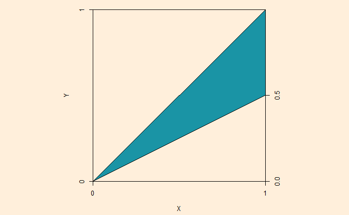
Now, here is a question. If A and B are two random points between 0 & 1, what is the probability A / B lies between 1 and 2?
We have seen how dice values are expressed as polynomials and how the resulting exponents become the sum and coefficients become the number of ways of obtaining the sum. Let’s extend this further and use dice rolling as a technique to estimate the production of polynomials.
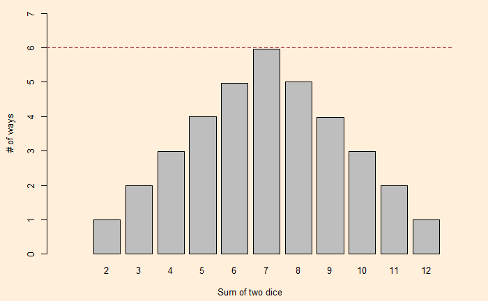
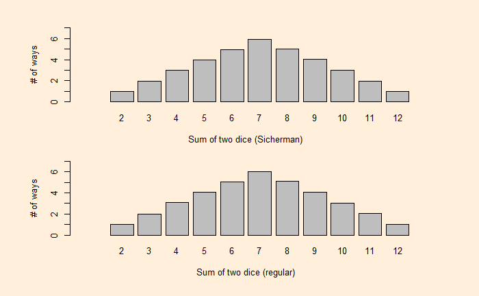
We have seen how one can describe a die with a polynomial. As a well-known example, i.e., the roll of two (regular) dice. The expected probabilities on the sum of dice are:
Where the exponents of x are the X-values and coefficients of x are the Y-values.
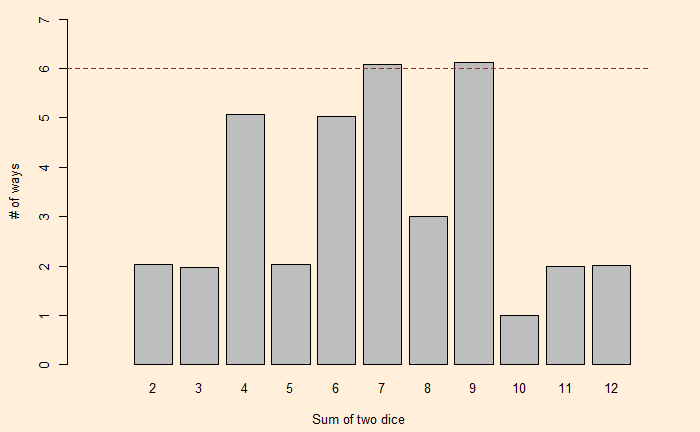
Now, a question arises: Can we find another pair of two dice with the same distribution for the sums? One way to find out is to factorise the polynomial, x12 + 2x11 + 3x10 + 4x9 + 5x8 + 6x7 + 5x6 + 4x5 + 3x4 + 2x3 + x2. George Sicherman discovered that another pair of numbers can lead to the same outcome. They are:
If n letters are placed randomly into n envelopes (with address), what is the expected number of envelopes with the correct letter inside?
Before addressing that, let’s look at a derangement problem. It is the probability of no match. For n items, it is the number of derangements divided by the number of permutations.
!n/n! = (n!/e)/n! ~ 1/e = 0.37
Let’s do a Monte Carlo and see what we get
itr <- 100000

let_env <- replicate(itr, {

  n <- 100

  env <- seq(1:n)
  let <- sample(seq(1:n), n, replace = FALSE, prob = rep(1/n, n))

  counter <- 0
for (i in 1:n) {
  if(env[i] == let[i]){
    counter <- counter + 1
  }else{
    counter <- counter
  }
}

  if(counter == 1) {
    sounder <- 1
  }else{
    sounder <- 0
  }


})

mean(let_env)
0.36827
So what about the original question of the expected number?
itr <- 100000

let_env <- replicate(itr, {

  n <- 100
  #env <- sample(seq(1:n), n, replace = FALSE, prob = rep(1/n, n))
  env <- seq(1:n)
  let <- sample(seq(1:n), n, replace = FALSE, prob = rep(1/n, n))

  counter <- 0
for (i in 1:n) {
  if(env[i] == let[i]){
    counter <- counter + 1
  }else{
    counter <- counter
  }
}

 counter
})

mean(let_env)
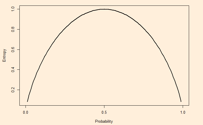
We have seen how the entropy of a system is derived as the surprise element of a system. The higher the entropy, the higher the surprise, ignorance or the degree of disorder of the system.
As an extreme example, the entropy of a double-headed coin is zero as it contains no information, i.e., always lands on heads!
On the other hand, a fair coin (50-50) produces a non-zero entropy. The full spectrum of entropy for a coin toss is:
Entropy is a concept in data science that helps in building classification trees. The concept of entropy is often explained as an element of ‘surprise’. Let’s understand why.
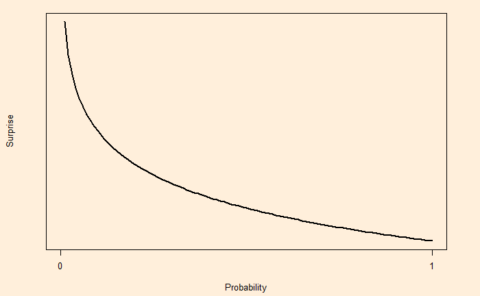
Suppose there is a coin that falls on heads nine out of ten or the probability of heads, p(H) = 0.9. So, if one tosses the coin and gets heads, it is less of a surprise as we expect it to show this outcome more often. whereas when it shows a tail, it is more surprising. In other words, surprise is somewhat an inverse of the probability, i.e. S = 1/p. But that has a problem.
If the probability of something is 1 (100% certain), 1/p becomes 1/1 = 1. Since we know the chance of that outcome is 100%, it should not be a surprise at all, but we get 1. To avoid that situation, S is defined as log (1/p). p = 1; S = log (1/1) = 0. On the other hand, p = 0; S = log(1/0) = log(1) – log(0) = undefined.
It is a practice to use log base 2 for calculating surprise for two outputs.
Surprise = log2(1 / Probability)
Now, let’s return to the coin with a 0.9 chance of showing heads. The surprise for getting heads is log2(1/0.9) = 0.15 and log2(1/0.1) = 3.32 for tail. As expected, the surprise of getting the rarer outcome (tails) is larger.
If the coin is flipped 100 times, the expected value of heads = 100 x 0.9 and the expected value of tails = 100 x 0.1. The total surprise of heads = 100 x 0.9 x 0.15 The total surprise of tails = 100 x 0.1 x 3.32 The total surprise = 100 x 0.9 x 0.15 + 100 x 0.1 x 3.32 The total surprise per flip = (100 x 0.9 x 0.15 + 100 x 0.1 x 3.32)/100 = 0.9 x 0.15 + 0.1 x 3.32 = 0.47
This is entropy – the expected value of the surprise.
Motivated reasoning is the tendency to favour conclusions we want to believe despite substantial evidence to the contrary. A famous example is climate change. In the US, for example, Democrats and Republicans disagree on the scientific consensus. A recent Pew Research survey on climate change presents the magnitude of this divide.
Prioritise alternative energy
At the highest level, 67% of people support this view, which is pretty impressive. But that is 90% Democrats (and Democrat-lining) and 42% Republicans (and leaning). The only silver lining is that 67% of Republicans under age 30 support alternative energy developments.
Climate change – a major threat to the well-being
Here again, the difference between the two parties is stark. In the last 13 years, the views from the Democrats have steadily increased from 61% to 78%, acknowledging climate change as a major threat. It has remained steady and low for the Republicans – at 25% in 2010 and 23% in 2022. Interestingly, 81% of French and 73% of Germans regard it a threat.

![\\ H = \sum\limits_{x=0}^{n} p(x) log_2[\frac{1}{p(x)}] \\\\ = 1 * log_2[\frac{1}{1}] + 0 * log_2[\frac{1}{0}] = 0](https://thoughtfulexaminations.com/wp-content/ql-cache/quicklatex.com-71946fe8b18e9e4a7d355da917b21654_l3.png "Rendered by QuickLaTeX.com")