A company has bought three software packages for their operations. They are Abacus, Biscuit and Circuit. On average, Abacus crashes 1 in 200 times, Biscuit 1 in 10 times, and Circuit 1 in 50. Of the ten employees, two were assigned Abacus, five got Biscuit, and three received Circuit. If Sophia’s trial crashed on the first trial, what is the probability that she got Abacus?
We have seen how the cap and trade works. The regulator sets a maximum value for the emissions (cap). It provides allowances, in emission permits, to firms to cover each unit of CO2 (or a pollutant) produced. The company can redeem one for every emission unit or trade it to another party, who can then use it.
Additionality is a term that is closely associated with this. By trading, an emitter can buy offset rather than reduce the emission. A quality offset must mean that GHG reduction has happened by the seller as a result of a project which otherwise would not have been possible. The additionality is a positive intervention that reduces GHG. In other words, it is not additional if the reductions would have happened anyway.
An infamous example is a company that declares offset by buying credits from a project that claims to conserve a forest which was already conserved!
If a 1-dimensional random walk starts at 0, with steps of one (to the right or left), what is the probability of reaching -30 before reaching 10?
Suppose P30 is the probability of reaching -30, and (1−P30) is the probability that to end with 10.
Let X be the position on the x-axis at the end of this game E[X] = -30 x P30 + 10 x (1-P30) For a random walk with equal steps (+1 or -1), E[X] = 0. 0 = -30 x P30 + 10 x (1-P30) -10 = P30(-30 -10) P30 = 1/4 = 0.25 = 25%
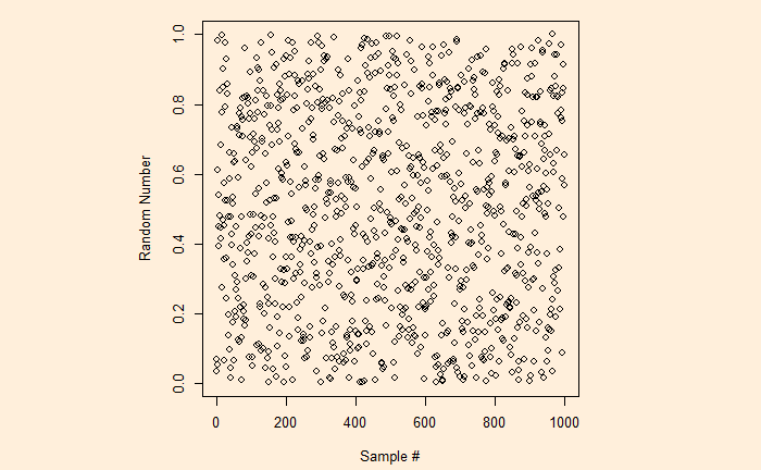
We know the ‘sample’ function creates a random sample of elements from a vector. But if you want to get a random sample between two limits, ‘runif’ is the function. Here is a plot of 1000 samples between 0 and 1.
runif(1000, min = 0, max = 1)
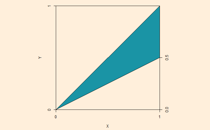
Now, here is a question. If A and B are two random points between 0 & 1, what is the probability A / B lies between 1 and 2?
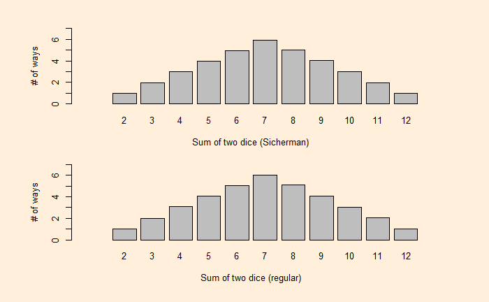
We have seen how dice values are expressed as polynomials and how the resulting exponents become the sum and coefficients become the number of ways of obtaining the sum. Let’s extend this further and use dice rolling as a technique to estimate the production of polynomials.
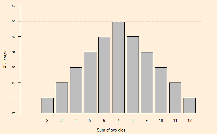
We have seen how one can describe a die with a polynomial. As a well-known example, i.e., the roll of two (regular) dice. The expected probabilities on the sum of dice are:
Where the exponents of x are the X-values and coefficients of x are the Y-values.
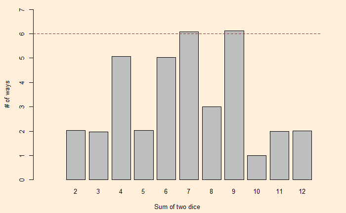
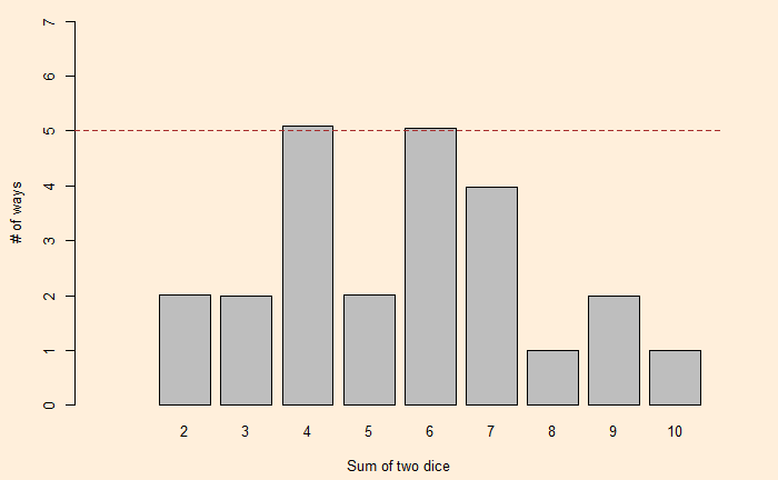
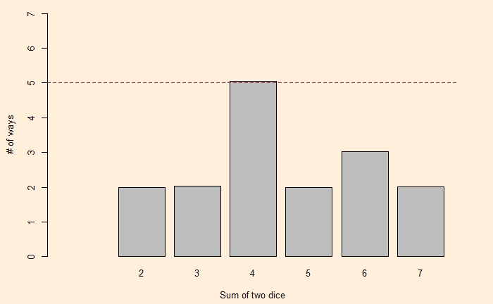
Now, a question arises: Can we find another pair of two dice with the same distribution for the sums? One way to find out is to factorise the polynomial, x12 + 2x11 + 3x10 + 4x9 + 5x8 + 6x7 + 5x6 + 4x5 + 3x4 + 2x3 + x2. George Sicherman discovered that another pair of numbers can lead to the same outcome. They are:
Well, I don’t think there is anything wrong with it! They are like the carbon tax and the cap and trade – means to charge the emitter their share of the social cost of carbon.
But what are fuel standards? These are regulations set by the government targeting to cut down CO2 emissions. For example, the US CAFE standards (corporate average fuel economy) required each manufacturer to meet two specified fleet average fuel economy levels for cars and light trucks, respectively. California pioneered the low carbon fuel standard that regulates the average carbon content per gallon of gasoline. If the former controls the amount one can burn, the latter focuses on capping the CO2 in the given amount of fuel.
Let’s understand how a fuel efficiency standard operates.
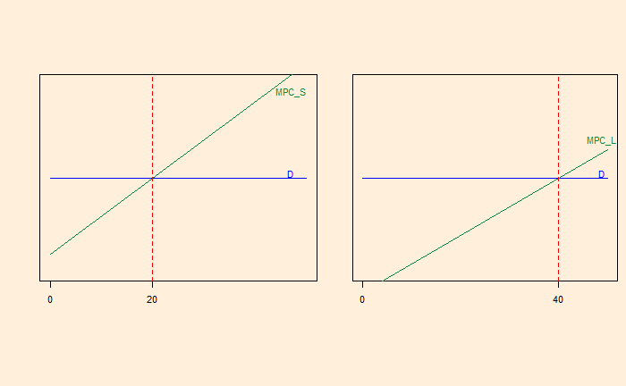
Suppose a manufacturer sells 20 small cars (S) and 40 large cars (L). Let the economies of these cards be 30 miles per gallon (mpg) for S and 10 mpg for L. The administration requires the average mpg (of the car sold) to be 20 mpg. On a simplistic level, this allows the company to sell one S for every L [(30 + 10) / 2 = 20 mpg]. Let’s look at a simplified supply-demand curve.
MPC = Marginal Private Cost or the change in the producer’s total cost brought about by the production of an additional unit. The flat demand curve means it is perfectly competitive.
Naturally, this must change as per regulation because the average mpg is (20 x 30 + 40 x 10) / 60 = 16.7; less than 20. One solution is to reduce L production to 20 and bring the mpg to the compliance level.
The shaded triangle on the right is the amount of profit that is forfeited in this exercise. What happens if I sell five more Ls? It would mean the company must sell five more Ss at a loss.
This process can go on until the red-shaded area on the left matches with the green-shaded area on the right. That means the S car sales increase.
So, a performance standard subsidises the product, which makes the standard easier. In other words, the firm taxes the poor-performing car by subsidising the better performer. The plot will tell you that L is sold at a price higher than its marginal cost, whereas S is sold below its marginal cost.
So, what is wrong with fuel standards? There is a possibility that the firm ends up selling more cars than it would do otherwise. There is also a possibility for the Jevons paradox, where people end up driving the fuel-efficient car more (rebound).
If n letters are placed randomly into n envelopes (with address), what is the expected number of envelopes with the correct letter inside?
Before addressing that, let’s look at a derangement problem. It is the probability of no match. For n items, it is the number of derangements divided by the number of permutations.
!n/n! = (n!/e)/n! ~ 1/e = 0.37
Let’s do a Monte Carlo and see what we get
itr <- 100000

let_env <- replicate(itr, {

  n <- 100

  env <- seq(1:n)
  let <- sample(seq(1:n), n, replace = FALSE, prob = rep(1/n, n))

  counter <- 0
for (i in 1:n) {
  if(env[i] == let[i]){
    counter <- counter + 1
  }else{
    counter <- counter
  }
}

  if(counter == 1) {
    sounder <- 1
  }else{
    sounder <- 0
  }


})

mean(let_env)
0.36827
So what about the original question of the expected number?
itr <- 100000

let_env <- replicate(itr, {

  n <- 100
  #env <- sample(seq(1:n), n, replace = FALSE, prob = rep(1/n, n))
  env <- seq(1:n)
  let <- sample(seq(1:n), n, replace = FALSE, prob = rep(1/n, n))

  counter <- 0
for (i in 1:n) {
  if(env[i] == let[i]){
    counter <- counter + 1
  }else{
    counter <- counter
  }
}

 counter
})

mean(let_env)
We have seen how the entropy of a system is derived as the surprise element of a system. The higher the entropy, the higher the surprise, ignorance or the degree of disorder of the system.
As an extreme example, the entropy of a double-headed coin is zero as it contains no information, i.e., always lands on heads!
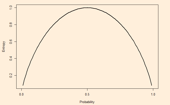
On the other hand, a fair coin (50-50) produces a non-zero entropy. The full spectrum of entropy for a coin toss is:
Entropy is a concept in data science that helps in building classification trees. The concept of entropy is often explained as an element of ‘surprise’. Let’s understand why.
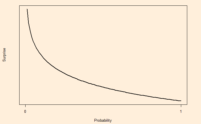
Suppose there is a coin that falls on heads nine out of ten or the probability of heads, p(H) = 0.9. So, if one tosses the coin and gets heads, it is less of a surprise as we expect it to show this outcome more often. whereas when it shows a tail, it is more surprising. In other words, surprise is somewhat an inverse of the probability, i.e. S = 1/p. But that has a problem.
If the probability of something is 1 (100% certain), 1/p becomes 1/1 = 1. Since we know the chance of that outcome is 100%, it should not be a surprise at all, but we get 1. To avoid that situation, S is defined as log (1/p). p = 1; S = log (1/1) = 0. On the other hand, p = 0; S = log(1/0) = log(1) – log(0) = undefined.
It is a practice to use log base 2 for calculating surprise for two outputs.
Surprise = log2(1 / Probability)
Now, let’s return to the coin with a 0.9 chance of showing heads. The surprise for getting heads is log2(1/0.9) = 0.15 and log2(1/0.1) = 3.32 for tail. As expected, the surprise of getting the rarer outcome (tails) is larger.
If the coin is flipped 100 times, the expected value of heads = 100 x 0.9 and the expected value of tails = 100 x 0.1. The total surprise of heads = 100 x 0.9 x 0.15 The total surprise of tails = 100 x 0.1 x 3.32 The total surprise = 100 x 0.9 x 0.15 + 100 x 0.1 x 3.32 The total surprise per flip = (100 x 0.9 x 0.15 + 100 x 0.1 x 3.32)/100 = 0.9 x 0.15 + 0.1 x 3.32 = 0.47
This is entropy – the expected value of the surprise.


![\\ H = \sum\limits_{x=0}^{n} p(x) log_2[\frac{1}{p(x)}] \\\\ = 1 * log_2[\frac{1}{1}] + 0 * log_2[\frac{1}{0}] = 0](https://thoughtfulexaminations.com/wp-content/ql-cache/quicklatex.com-71946fe8b18e9e4a7d355da917b21654_l3.png "Rendered by QuickLaTeX.com")