April 2023

German Tank Problem

The German tank problem is about the math that helped the Allies in WW2 to estimate the number of German tanks (panther) based on the ‘samples’, i.e., the ones captured. In a war, an accurate estimate of the maximum number of tanks on the enemy side helps estimate the size of the threat.

The Allies discovered that the components of the tanks had sequential serial numbers. Then they assumed that the probability of finding any tank from #1 to #N (the maximum) was equally distributed (uniform distribution) at 1/N. The serial numbers of the captured tanks then gave them the samples.

Imagine at some stage, the following five tanks were captured: 15, 47, 79, 28, 39. Organising them in increasing order, we get 15, 28, 39, 47, 79. We will consider them as random draws from the uniform distribution and calculate the gaps between them without taking the numbers themselves. They are 14, 12, 10, 7 and 31. The average of these gaps = 14.8. Add this correction factor to the maximum number 79 to get 94.

If m is the highest number, k is the number of tanks captured, and N is the (unknown) total number,

N = m + m/k – 1

Reference

German tank problem: Wiki

German Tank Problem Read More »
Blood-Pressure Control: SPRINT Study

The SPRINT study, sponsored by The National Heart, Lung, and Blood Institute, has been a landmark work which affirmed the value of keeping systolic pressure at a lower level through intensive treatment. SPRINT is the acronym for Systolic Blood Pressure Intervention Trial that compared the benefit of maintaining systolic blood pressure < 120 mm Hg with treatment for < 140 mm Hg.

SPRINT study enrolled 9361 participants above 50 years with high blood pressure (130 to 180 mm Hg), but without diabetes, between 2010 through 2013. SPRINT was a randomized, controlled, open-label trial that compared the study outcomes between the standard-treatment group (systolic blood-pressure target < 140 mm Hg) and the intensive-treatment group (systolic blood pressure target < 120 mm Hg).

A committee of professionals, unaware of the study-group assignments, judged the medical outcomes of the participants. The primary composite outcome was myocardial infarction, other acute coronary syndromes, stroke, heart failure, or death from cardiovascular causes. Secondary outcomes included the individual components of the primary composite outcome, death from any cause, and the composite of the primary outcome or death from any cause.

The results

Key results are summarised below

OutcomeIntensive
Treatment

(N = 4678)
Standard
Treatment

(N = 4683)
Hazard
Ratio
p-value
Primary
outcome
2433190.75<0.001
Death from
cardiovascular
causes
37650.570.005
Myocardial
infarction
971160.780.19
Stroke62700.470.5
Death from
any cause
1552100.730.003

Reference

A Randomized Trial of Intensive versus Standard Blood-Pressure Control: NEJM

Blood-Pressure Control: SPRINT Study Read More »

Tennis Player’s Dilemma

An upcoming tennis player can win a prize if she wins two consecutive matches in a three-game series against the #1 and #2 players alternately. She can choose either of the matchups: 121 or 212. Which scheme has a better chance of winning the prize?

Let p1 be her chance to defeat #1 and p2 to beat #2; p1 < p2 (#1 is a better player than #2).

Matchup 121

The probability of winning two consecutive matches in the 121 scheme is: p1 x p2 x p1 + p1 x p2 x (1-p1) + (1-p1) x p2 x p1 = p1p2(2 – p1)

Matchup 212

The probability of winning two consecutive matches in the 212 scheme is: p2 x p1 x p2 + p2 x p1 x (1-p2) + (1-p2) x p1 x p2 = p1p2(2 – p2)

Therefore, it reduces to a comparison bewteen p1p2(2 – p1) vs p1p2(2 – p2) or (2-p1) vs (2-p2).

Since p1 < p2, (2-p1) > (2-p2). So she must go for matchup 121.

Reference

Fifty Challenging Problems In Probability: Frederick Mosteller

Tennis Player’s Dilemma Read More »

Flippant Juror Problem

There are two systems of the jury. The first is a 1-member jury with a probability p to deliver the correct verdict. The second system is a 3-member jury that works on majority (at least 2) decisions to win. The two members each have an independent probability, p, for making the correct decision, and the third juror flips a coin and decides. Which jury has a better chance of making the right decisions?

Take the case of the 3-member jury:

The probability of getting the majority right = P(all three right) + P(first two correct AND third wrong) + P(first and third right AND second wrong) + P(second and third right AND first wrong)

= p x p x 1/2 + p x p x 1/2 + p x 1/2 x (1-p) + p x 1/2 x (1-p)

= (1/2) x (p2 + p2 + p – p2 + p – p2)

= 2p/2 = p = probability of 1-member jury to make the correct decision.

Flippant Juror Problem Read More »

Cardano’s Games of Chance

How many throws of a fair are required to have an even chance of at least one six?

Let’s break down the problem. 1) The probability of at least one six in n throws is (1 – the probability of getting no sixes in n throws). It is 1 – (5/6)n. 2) Even chance means 0.5. By combining the two pieces of information:

1 – (5/6)n = 0.5

Taking logs on both sides,

n ln (5/6) = ln(1/2)
n = ln(1/2)/ln (5/6) = 3.8

So, four throws.

Cardano’s Games of Chance Read More »

Newton-Pepys Problem

Ana, Betty and Carol are doing a competition. Ana can throw a die six times and aims to get at least one ‘6’. Betty can throw twelve times but needs to get at least two 6s. Carol has eighteen chances to get at least 3. Who has a better chance of winning the competition?

Let’s calculate the chances of each using binomial trials.

the probability of s successes in n rounds is nCs x ps x q(n-s)

Ana’s chances

The probability of getting at least one 6 in 6 tries is (1 – the probability of getting no success)

1 – 6C0 x (1/6) 0 x (5/6)(6-0) = 0.665

Betty’s chances

The probability of getting at least two 6s in 12 tries is (1 – the probability of getting no success – the probability of getting one success).

1 – 12C0 x (1/6) 0 x (5/6)(12-0)12C1 x (1/6) 1 x (5/6)(12-1) = 0.619

Carol’s chances

The probability of getting at least three 6s in 18 tries is (1 – the probability of getting no success – the probability of getting one success – the probability of getting two success).

1 – 18C0 x (1/6) 0 x (5/6)(18-0)18C1 x (1/6) 1 x (5/6)(18-1)18C2 x (1/6) 2 x (5/6)(18-2) = 0.597

Newton-Pepys Problem Read More »

Park Run Bingo

Suppose Ana wants to participate in a park run bingo – a version of what is known as stop-watch bingo – how many weekends is she expected to run to tick off the whole card?

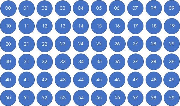
In a stopwatch bingo, one tick off on the card, the digits (00-59), the seconds that show up on the watch. So for a weekly park run, it could be the seconds of the final timing recorded by the organiser. Notice if you take down timings from your watch, it becomes challenging to maintain randomness.

If you apply the formulation that we did in the earlier post, you get,

E(T) = 60*[1 + \frac{1}{2} + \frac{1}{3} + ... + \frac{1}{60}]

nn <- 60
run.sum <- rep(0, nn)
run.sum[1] <- 1.0
for(i in 2:nn){
current = nn/(nn - i +1)
run.sum[i] <- run.sum[i-1] + current
}
run.sum[nn]

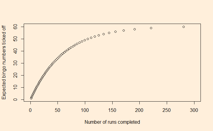
The answer is 281.

You can see from the graph that by about 50 runs, you could be getting close to 40 unique numbers; it then becomes difficult to avoid duplications.

The Coupon Collector’s Problem: Stand-up Maths

Coupon collector’s problem: Wiki

Park Run Bingo Read More »

NBA Draft Lottery – More Stats

Having seen the probability of winning the lottery picks in the NBA, it would be interesting to see how fortune has favoured the teams historically. Last year (2022), the top four went to, respectively, Magic (2nd), Okc (4th), Rockets (1st) and Kings (7th). So, the number 7 got a lift of 3 places and reached inside top 4. It’s a coincidence that the 7th team has been in the lottery pick every year since 2018! Well, the odds of the 7th team getting inside the lottery (top 3 then) had been 16% in 2018 and 32% since then.

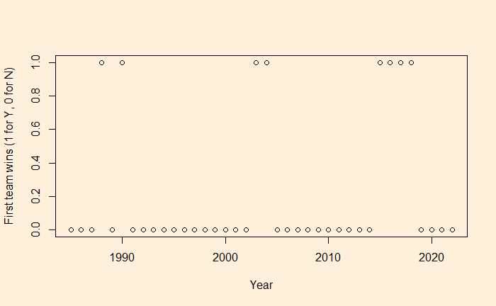
But how many times the first draw has gone to the top 1 team (i.e., the last one of the regular season)? Here is the graph summarising the statistics from 1985 through 2022.

Here ‘1’ means if the first team got the first pick and ‘0’ otherwise.

Note that the probability for the first team to come first in the lottery has changed over the year – 14.29 in the first four years, followed by 11.11 for a year, then 16.7, 25 for a long time until the latest 14% since 2019. Considering all these, the average probability of winning first is 21.48%. And the eight winners in the last 38 years suggest the actual data stands at 21%!

In 1993, the Orlando Magic got the first pick, whereas its pre-lottery chance was merely 1.52%. Similar things happened in 2008 (1.70%, Chicago Bulls) and 2014 (1.70%, Cleveland Cavaliers). The Cavaliers have more instances of luck, where they got Kyrie traded from the Clippers in 2011, where the latter had a 2.8% chance to win the first draw, and the ultimate price, Lebron James in 2003, where they were indeed the first one on the list!

References

NBA Draft Lottery History: Real GM
Tanking Won’t Die in the New NBA Draft Lottery System: The Ringer
NBA Draft Lottery: NBA
Top 5 NBA Draft Lottery Miracles: NBC

NBA Draft Lottery – More Stats Read More »

Flipping Biased Coins

After a break, we are back with coin-flipping games. Here is the first – A biased coin produces heads 70% of the time. You toss the coin twice. If both tosses have the same outcome, what is the probability that both tosses are tails?

Let’s apply the general form of Bayes’ equation straightaway.

P(TT|Same) = \frac{P(Same|TT) * P(TT)}{P(Same|TT) * P(TT) + P(Same|HT) * P(HT) + P(Same|TH) * P(TH) + P(Same|HH) * P(HH)} \\ \\ =  \frac{1 * 0.3*0.3}{1 * 0.3*0.3 + 0 + 0 + 1 * 0.7*0.7} = \frac{0.09}{0.58} = 0.155 \\ \\

Second one: there are two kinds of coins in a box in equal numbers – fair coins and the biased coins of the previous type (70% heads). You randomly select one and flip it twice. If it lands tails on both occasions, What is the probability that the coin is biased?

P(Biased|TT) = \frac{P(TT|Biased) * P(Biased)}{P(TT|Biased) * P(Biased) + P(TT|NOT-Biased) * P(NOT-Biased)} \\ \\ =  \frac{0.3*0.3*0.5}{0.3*0.3*0.5+ 0.5*0.5*0.5} = \frac{0.045}{0.17} = 0.265 \\ \\

Flipping Biased Coins Read More »

The Coupon Collector Problem

Imagine that a person wants to collect coupons that come along with a product. Each product pack can contain one of the ten types of coupons, and her goal is to accumulate all of them. The question is: how many packets does she need to open to get all ten coupons?

Remember the post on expected waiting time? It says: if something has a probability p to occur, the amount of time you wait 1/p. It is the expected waiting time. So, start our problem in steps.

The probability of getting a new coupon from the first purchase is 10/10 = 1. The expected time or the number of packets to open is 1/1 = 1, which is not surprising. Note that it is a problem with replacement, i.e., the same type of coupon can come again. What is the probability of getting a new card the next time? It’s given by dividing the number of ‘not-yet-collected’ coupons / by the total number of coupons = 9/10. Naturally, the expected time gets longer = 10/9. Finally, when you got everything but the last, it requires 10/1 or ten purchases for the elusive one!

The total time required is the time to get the first coupon + the additional time for the second + third + … 10. It is 1 + 10/9 + 10/8 + 10/7 + 10/6 + 10/5 + 10/4 + 10/3 + 10/2 + 10/1 = 10 (1/10 + 1/9 + …. 1). Rearranging this will make it familiar: 10 (1 + 1/2 + 1/3 + 1/4 + 1/5 + 1/6 + 1/7 + 1/8 + 1/9 + 1/10).

In general, for N coupons, it becomes N x (1 + 1/2 + …. 1/N) = N x HN. And HN is the Nth Harmonic number. From the wiki, the approximation for the sum equals,

\\ E(T) = N * H_N = N*ln(N) + \gamma*N + 1/2 + O(1/N)\\ \\ \gamma = 0.577

So, for the 10-coupon problem. she may be purchasing, on average, 29 packs of the product!

Coupon collector’s problem: Wiki

The Coupon Collector Problem Read More »