Science

Chi-square – Interpretation

Un-VaccinatedVaccinated
(O-E)2/E(O-E)2/E
Contracted
pneumococcal pneumonia
5.785.78
Contracted
another type of pneumonia
0.110.11
Did not contract pneumonia0.930.93

You can see that the largest numbers for the chi-squares are against the row: ‘Contracted pneumococcal pneumonia’. These mean the largest departure from the expected values.

Un-VaccinatedVaccinated
(O-E)2/E(O-E)2/E
Contracted
pneumococcal pneumonia
(23 – 28*92/184)2/
(28*92/184)
(5 – 28*92/184)2/
(28*92/184)
Contracted
another type of pneumonia
(8 – 18*92/184)2/
(18*92/184)
(10 – 18*92/184)2/
(18*92/184)
Did not contract pneumonia(61 – 138*92/184)2/
(138*92/184)
(77 – 138*92/184)2/
(138*92/184)

In the unvaccinated case, the observation was more than the expectations (O:23 vs. E:14), whereas in the vaccinated case, it was fewer (O:5 vs. E:14).

Smaller values of chi-square suggest observed values are closer to the expected.

Reference

The Chi-square test of independence: Biochem Med 

Chi-square – Interpretation Read More »
Chi-square for Science

Science is built on the foundations of hypothesis testing. The Chi-square test of independence is one prime statistic for testing hypotheses when the variables are nominal.

The application of the Chi-square test is widely prevalent in clinical research. Here is an example of a case study published in ‘Biochemia Medica’. Following is the data from a group of 184 people, half of whom received a vaccine against pneumococcal pneumonia.

Un-VaccinatedVaccinated
Contracted
pneumococcal pneumonia
235
Contracted
another type of pneumonia
810
Did not contract pneumonia6177

1. Marginals

The first step in the Chi-square test is the calculation of the ‘marginals’. As marginals mean ‘on the sides’, we write them on the right column (the row-sums) and the bottom row (the column-sums).

Un-VaccinatedVaccinatedRow Sum
Contracted
pneumococcal pneumonia
23528
Contracted
another type of pneumonia
81018
Did not contract pneumonia6177138
Column Sum9292N = 184

2. Expected values

The chi-square test requires observed and expected values. It applies the following formula to each element and adds them up.

(O-E)2/E

The observed values are the data, and expectations are to be estimated based on the marginals. The expected data for a perfectly independent scenario is calculated as below. The expected value at (row i, column j) is obtained by RowSum(i) x ColumnSum(j)/(N).

Un-VaccinatedVaccinated
(O-E)2/E(O-E)2/E
Contracted
pneumococcal pneumonia
(23 – 28*92/184)2/
(28*92/184)
(5 – 28*92/184)2/
(28*92/184)
Contracted
another type of pneumonia
(8 – 18*92/184)2/
(18*92/184)
(10 – 18*92/184)2/
(18*92/184)
Did not contract pneumonia(61 – 138*92/184)2/
(138*92/184)
(77 – 138*92/184)2/
(138*92/184)

3. Test for Independence

Un-VaccinatedVaccinated
(O-E)2/E(O-E)2/E
Contracted
pneumococcal pneumonia
5.785.78
Contracted
another type of pneumonia
0.110.11
Did not contract pneumonia0.930.93

The Chi-square is calculated as the overall sum = 13.649

The p-value is estimated by looking at the Chi-square table for 13.349 at degrees of freedom (df) = 2.

The R code for the whole exercise

edu_data <- matrix(c(23, 5, 8, 10, 61, 77), ncol = 2 , byrow = TRUE)
colnames(edu_data) <- c("Vac", "No-Vac")
rownames(edu_data) <- c("npneumococcal pneumonia", "non-pneumococcal pneumonia", "Stayed healthy")


chisq.test(edu_data)
edu_data
	Pearson's Chi-squared test

data:  edu_data
X-squared = 13.649, df = 2, p-value = 0.001087

                           Vac No-Vac
npneumococcal pneumonia     23      5
non-pneumococcal pneumonia   8     10
Stayed healthy              61     77

The p-value suggests that the impact of vaccination on protecting against pneumococcal pneumonia is significant. And there is only a 1.1 in a thousand possibility that the difference is out of pure chance.

Reference

The Chi-square test of independence: Biochem Med 

Chi-square for Science Read More »

Turn of the knob

Came across one of the finest videos on YouTube about our past, present and future life, Yuval Noah Harari’s talk to youngsters and teachers, which triggered the idea of this post.

Turning the knob

Knowledge is like turning the knob. When it turns, you see things in a new light; until then, no matter how hard you try, you don’t get it out of ‘common knowledge’. Unfortunately, the common knowledge is almost always wrong!

The hyperpigmented on the equator

Take the favourite example of pigmentation of humans living in the equatorial region. For a moment, let’s ignore the people who believe that people of colour are of a separate species. We are dealing with more reasonable people here. If the narrative is that people in sunny regions have become dark-skinned because of heat and light, it’s an easier narrative to sell. It fits with the common knowledge – we all know what happens when we fry things; a little too much and it turns black.

Unfortunately, that’s not how things evolve. The theory of evolution switch needs to turn on. What about this: a group of people (perhaps dominated by the light-skinned) reach a sunny region. A few of them got skin cancer due to their lack of protective pigmentation and died maybe a few years earlier than their accidentally darker companions. That raised (by a small margin) the probability of darker parents, their children and their children having the advantage, and wow, after 10,000 years, there was a complete dominance of the dark. So, will that happen in Australia after 10,000 years? We’ll answer that in the end.

Humans of Flores

There used to be a pack of humans living in Flores, an island in Indonesia (until they were extinct about 50,000 years ago). They were humans as they shared the homo family. They were different humans because we are homo sapiens, and they were not. They were pretty short – about 1 m. tall – people. Not just them but the animals of that island as well. A simple convincing argument is that the animals got trapped on the island, became resource-constrained, and to survive, they had to consume less food. And they became smaller. It’s convincing because 1) it gives a feeling that one bunch of people after starvation has shrunk, or 2) they passed a genetic code to the children and made them shrink.

Turn the switch, and you get it: big humans reached the island. Once they got disconnected from the mainland due to sea level rise, the larger ones faced a more significant disadvantage due to food shortage, and the smaller ones survived better. In the next generation, there were disproportionally smaller kids from the surviving parents (the new group has larger ones too). Turn a few pages, centuries and generations: the island is full of smaller humans. This narrative is difficult to fathom without the switch as it is against the common knowledge. First, how can more miniature humans be fitter? That doesn’t conform very well with the stereotypes! Second, something forcing people (in one lifetime) to become smaller is easier to imagine than this chance game of smaller ones surviving (in a hundred lifetimes).

The future evolutions

That naturally begs the question. Will the Australians (the white Australians) turn back after 10,000 years? Even the broader question: What will be the next evolution of humans? The answer to the first question is a no, and the answer to the second question is impossible to predict.

The code lies in the knowledge paradox we are in. Australian whites won’t turn black because they know why it happens and what to do against death from skin cancer. It could be as simple as using sunscreen (or deciding not to venture out in the UV-intense part of the day). And this will translate to other things as well. If we know something gives us a disadvantage, we will engineer means to counter it. It has to be a disadvantage that gave the survivors the chance to survive, and we are closing those weaknesses!

Must watch video

Yuval Noah Harari Speaks to Young Readers & Teachers: Yuval Noah Harari

Turn of the knob Read More »

The Science We Trust

People lament about the dominance of beliefs and the reduction of scientific temperament in society. Unfortunately, it is a fact and can only be worse in future. And I want to argue that it can only be like that. Let’s look at a few reasons why achieving scientific character is a mission impossible.

It’s another religion

Unfortunately, it has to be.

Take the example of the discovery of gravitational waves in 2015. The number of people involved in the observation, which includes the setting hypothesis, the detection, and the mathematical modelling, could be about 1000. The rest of the world (1000 short of 7 billion) only gets the publication, which is already a heavily cut-down, readable version of the actual data.

Imagine a million people downloaded the paper.

As per an old report in physics today, the percentage of physics graduates (minimum decent training level in this field) was about 0.01. It suggests the inconvenient truth that 99.99% of people are already at a considerable disadvantage.

I.e., half all physics graduates and the rest others!

The people who understand the model (the specific mathematics behind the event) are even fewer and could be in the hundreds at best.

All the others – 6999 million out of 7000 – get the news from the media. And they must trust the report. A belief system is created but is not going to last like a religion, as we shall see soon.

What is Science

Most people know science through technology, the application of the former into products. To define it in one word: science is hypothesis testing. And most people are alien to it. It is probabilistic, conditional, and will/must update with time. Each of these contradicts the doctrines of religion.

Probabilistic thinkers meet the real people

Back to the gravitational waves: Movements on the ground, temperature changes in the instruments or numerous other known or unknown errors can all lead to artificial signals or noises. The importance of the results led to keeping a significance level for the rejection of the null hypothesis (that the observed signal is a noise) to be extremely low – one in a billion. If you recall, most of our ordinary life experiments that is one in 20!

The team investigating the gravitational waves published the findings (as real) only when they found the probability that it could happen by chance is one in a billion. Yet, they would only use the words such as ‘likely’, ‘probably’ or ‘mostly’, to respond to the public, who want ‘yes’ or ‘no’ as answers.

And they change with time

Science updates with new information. Remember the chaos during covid time? The understanding of the illness changed daily during the pandemic. The use of masks (to use or not to use) and modes of contagion (airborne vs liquid-borne), to name a few. While the changes of advice were perfectly understandable and acceptable for those scientists, it was causing confusion and anger to the 99.99%.

The Science We Trust Read More »

Drinking and Police

Here is some data on drinking and getting in trouble with the police. Assess the relationship between drinking habits and getting into trouble with the authorities. Does this data provide evidence of drinking and getting into trouble with the police?

NeverOccasionalFrequent
Trouble with Police 60200420
No trouble with Police 480027002800
Observation table

The first step is to form the hypothesis. Here is the null hypothesis:

H0 – Drinking habits and getting into trouble with the police are independent.

The alternative is

H1 – Drinking habits and getting into trouble with the police are not independent.

We will use the chi-squared test to validate the null hypothesis.

We will use the chi-squared test to validate the null hypothesis. It requires observed data as well as the expected data under the null hypothesis conditions. From the data, the number of people belonging to each of the drinking categories is:

NeverOccasionalFrequentTotal
#48602900322010980
%44.2626.4129.33100

So, under ‘normal’ conditions (conditions of independence), one would expect similar percentages of individuals getting into trouble with the police, the expected numbers we needed.

NeverOccasionalFrequent
Trouble with Police 301178200
No trouble with Police 455927203020
Expectation table

If you add a row below each category, you will get the same split as per the total.

NeverOccasionalFrequent
%44.2626.4129.33

It’s time for the chi-square test, i.e. (observed – expected)2/expected summed over all the members.

(60 – 301)2 / 301 + (200 – 178)2 / 178 + (420 – 200)2 / 200 +(4800 – 4559)2 / 4559 +(2700 – 2720)2 / 2720 + (2800 – 3020)2 / 3020 = 467

The chi-squared statistic is 467. The degrees of freedom are the product of one less than the number of categorical variables (i.e. (2-1) x (3-1) = 2). Upon looking at the probability table, you can find that 467 is way on the right side of the distribution, with the probability (p-value) almost zero. So the data did not happen by chance, and the null hypothesis is rejected.

Drinking and Police Read More »

An Ocean Full of Bombay Duck

Here is a story of the survival of the fittest. It seems it is caused by global warming or some other confounding factor. A recent publication by Kang et al. in “Environmental Biology of Fishes” tells a curious – potentially scary – case of things to come.

The team noticed a sudden spike in a particular variety of fish off the coast of southeast China. This weirdly named fish, the Bombay Duck, has had a ten-fold population growth in the last decade. Bombay Duck (Harpadon nehereus) is fish that can survive a low Oxygen environment due to a high (about 90%) water content in its tissues.  

So scientists postulate that as the water temperature rises, thanks to global warming, the dissolved oxygen levels in the water drop, and makes the lives of the indigenous fish species in danger, leaving only those species that can thrive under these conditions to multiply in numbers. So a fish that did not exist in the national statistics as an independent species until recently suddenly becomes a dominant variety.

Increase of a hypoxia-tolerant fish: Environmental Biology of Fishes

An Ocean Full of Bombay Duck Read More »

Physical Activity and Health

The March issue of the British Journal of Sports Medicine came out with the results from a 9-year-long cohort study of people who did physical activity and its impact on influenza and pneumonia.

Before we get into details, note that it is a cohort study – of 577 909 US adults. Cohort studies are observational, whereas randomised controlled trials (RCTs) are interventional. Establishing causations from observational studies is problematic.

A key finding of the study has been the association of lowered risk of influenza and pneumonia with aerobic physical activity.

Reference

Webber BJ, et al. Br J Sports Med 2023;0:1–8.

Physical Activity and Health Read More »

Blood-Pressure Control: SPRINT Study

The SPRINT study, sponsored by The National Heart, Lung, and Blood Institute, has been a landmark work which affirmed the value of keeping systolic pressure at a lower level through intensive treatment. SPRINT is the acronym for Systolic Blood Pressure Intervention Trial that compared the benefit of maintaining systolic blood pressure < 120 mm Hg with treatment for < 140 mm Hg.

SPRINT study enrolled 9361 participants above 50 years with high blood pressure (130 to 180 mm Hg), but without diabetes, between 2010 through 2013. SPRINT was a randomized, controlled, open-label trial that compared the study outcomes between the standard-treatment group (systolic blood-pressure target < 140 mm Hg) and the intensive-treatment group (systolic blood pressure target < 120 mm Hg).

A committee of professionals, unaware of the study-group assignments, judged the medical outcomes of the participants. The primary composite outcome was myocardial infarction, other acute coronary syndromes, stroke, heart failure, or death from cardiovascular causes. Secondary outcomes included the individual components of the primary composite outcome, death from any cause, and the composite of the primary outcome or death from any cause.

The results

Key results are summarised below

OutcomeIntensive
Treatment

(N = 4678)
Standard
Treatment

(N = 4683)
Hazard
Ratio
p-value
Primary
outcome
2433190.75<0.001
Death from
cardiovascular
causes
37650.570.005
Myocardial
infarction
971160.780.19
Stroke62700.470.5
Death from
any cause
1552100.730.003

Reference

A Randomized Trial of Intensive versus Standard Blood-Pressure Control: NEJM

Blood-Pressure Control: SPRINT Study Read More »

Three-parent baby

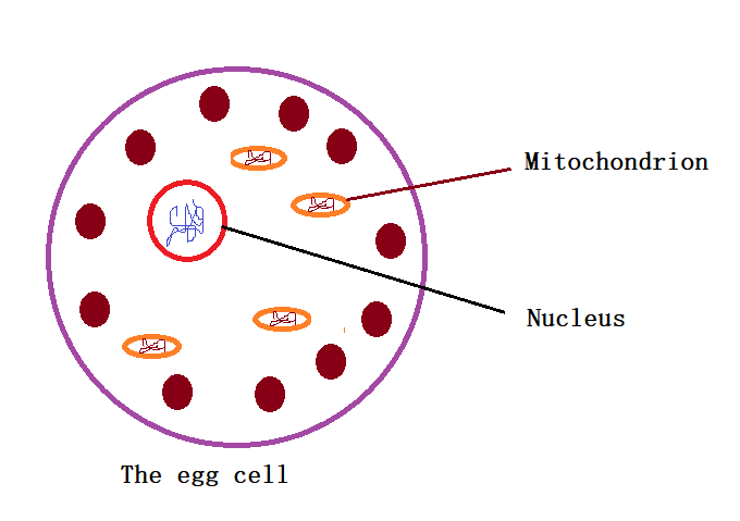
We have seen Mitochondrial DNA (mtDNA) as a valuable tracer to follow maternal ancestry. To take a step back: the majority of human DNAs reside inside the cell nucleus, and a few are inside another structure inside the cell, the mitochondrion. During reproduction (fusion of egg and sperm), nuclear DNA undergoes recombination with material from both parents participating, whereas mtDNA we possess entirely comes from the mother’s ovum. It happens due to the faster degradation of mitochondria from the sperm during fertilisation.

Leigh syndrome

Leigh syndrome is a fatal disorder, and its genes reside in the DNA of the mitochondria. If the mother has the disease, it’s sure to reach the offspring, jeopardising its health. In 2016 John Zhang’s team at the New Hope Fertility Center in New York City found a solution. They ‘swapped’ the mitochondria of the mother with a healthy donor.

The technique was to take a healthy donor egg, remove the (cell) nucleus and replace it with that from the mother. Scientists then fertilised the egg with the father’s sperm and implanted it into the mother’s womb. While the majority of the genetic material is from the mother and father, those from the mitochondria are from the donor, thus making her the ‘third parent’.

World’s first baby born with New “3-parent” Technique: New Scientist
The three-parent baby technique could create babies at risk of severe disease: MIT Technology Review

Three-parent baby Read More »

Rare Disease Revisited

Remember when we discussed the application of Bayes’ theorem to quantify the predictive values of medical tests? It gives the probability that a person has a (rare) disease, given she is tested positive. Today, we verify the solution using a simple R code by sampling a million people!

Using the familiar notations, we write down Bayes’ formula.

P(D|+) = \frac{P(+|D) P(D) }{P(+|D) P(D) + P(+|NoD) P(NoD)}

Let’s assign probabilities to each of the parameters.

1) The test shows positive 90% of the time on patients with the disease (high sensitivity); P(+|D)
2) The test shows negative 95% of the time on healthy patients (high specificity); P(-|noD)
3) The disease is present in 1% of the community (low prevalence ) P(D)

Note that specificity = P(-|noD), whereas what we want is P(+|NoD), which is 1 – P(-|noD). Substituting all values,

\\ P(D|+) = \frac{P(+|D) P(D) }{P(+|D) P(D) + P(+|NoD) P(NoD)} \\ \\ P(D|+) = \frac{Sensitivity *  Prevalence}{Sensitivity *  Prevalence + (1-Specificity)*(1- Prevalence)} \\ \\ P(D|+) = \frac{0.9*0.01}{0.9*0.01 + 0.05*0.99} = 0.15

Let’s develop a code that simulates the testing of a million people.

Step 1: A million people, with 1% (random) having the disease. 1 = disease, 0 = no disease.

disease <- sample(c(0,1), size=1e6, replace=TRUE, prob=c(0.99,0.01))

Step 2: Create an empty vector with a million slots.

test <- rep(NA, 1e6)

Step 3: Fill the disease columns (disease = 1) with random assignment of test results; 90% with 1 and 10% with 0.
Fill the nondisease columns (disease = 0) with random assignment of test results; 95% with 0 and 0.05% with 1.

test[disease==1] <- sample(c(0,1), size=sum(disease==1), replace=TRUE, prob=c(0.1, 0.9))
test[disease==0] <- sample(c(0,1), size=sum(disease==0), replace=TRUE, prob=c(0.95,0.05))

Now estimate the average number of people with disease = 1 AND test = 1.

mean(disease[test==1]==1)

Putting everything together,

disease <- sample(c(0,1), size=1e6, replace=TRUE, prob=c(0.99,0.01))
test <- rep(NA, 1e6)
test[disease==1] <- sample(c(0,1), size=sum(disease==1), replace=TRUE, prob=c(0.1, 0.9))
test[disease==0] <- sample(c(0,1), size=sum(disease==0), replace=TRUE, prob=c(0.95,0.05))
mean(disease[test==1]==1)

Rare Disease Revisited Read More »