Science

Bayes Factor – Continued

Let’s progress further the concept of Bayes Factor (BF). In the last post, the BF was defined in favour of the null hypothesis (BF01). From now on, we focus on BF10 or the Bayes factor in favour of the alternate hypothesis.

Bayes Factor10 = P(Data|H1) / P(Data|H0)

As per Bayes theorem:
P(H1|D) = [P(D|H1) P(H1)] / P(D)
P(H0|D) = [P(D|H0) P(H0)] / P(D)
[P(H1|D) / P(H0|D)] = [P(D|H1) P(H1)] / [P(D|H0) P(H0)]
[P(H1|D) / P(H0|D)] = [P(D|H1) / [P(D|H0)] [P(H1)] / P(H0)]
Posterior Odds = BF10 x Prior Odds

This definition is significant in determining the strength of the alternate hypothesis given the experimental data or P(H1|D). Note that an experimenter is always interested in it, but the traditional hypothesis testing and p-values never helped her to know it. Let’s see how it works:

Let the prior probability for your hypothesis be 0.25 (25%), which is 1:3 prior odds (note: P(H1) + P(H0) = 1 and P(H1|D) + P(H0|D) = 1). And the BF10 is 5, which is pretty moderate evidence and is not far from a p-value of 0.05. The posterior odds become 5:3 (P(H1|D) / P(H0|D)). This corresponds to a posterior probability for the alternate hypothesis (P(H1|D)) = 5/8 = 0.625 (62.5%).

So, a Bayes Factor of 5 has improved the prior probability of the hypothesis from 25% to 62.5%.

Bayes Factor – Continued Read More »
Bayes Factor

Most of the hypothesis testing we have seen so far comes under the category of what is known as the null hypothesis significance testing (NHST). In this framework, we have two competing hypotheses:

  1. The Null Hypothesis, H0, where there is no impact of an intervention
  2. Alternate Hypothesis, HA, where there is an impact of the intervention.

Hypothesis testing aims to collect data (evidence) and assess the fit for one of the above models. At the end of NHST, you either ‘reject’ or ‘fail to reject’ your Null hypothesis – at a specified significance value – using the well-known p-value.

p-value ~ P(Data|H0)

On the contrary, we can define a ratio that gives equal weightage for the null and the alternative hypotheses. That is the Bayes Factor. It compares the probability of the data under one hypothesis with the probability under the other.

Bayes Factor01 = P(Data|H0) / P(Data|H1)

If BF01 > 1, the data is likely supporting H0
If BF01 < 1, the data is likely supporting H1

Bayes Factor Read More »

Anthropic Principle

The anthropic principle says that in the universe, our presence as observers compels conditions for our presence. While the idea was not entirely new, the phrase came up in 1973 by Brandon Carter, who proposed the weak and strong forms of anthropic principle.

The weak anthropic principle (WAP) merely says that you need to take into account those things in the environment that you can see vs those things you are unable to see. Or it simply says that the life-free universes cannot be observed it’s just a selection bias.

An example is the cosmological constant (lambda). The number must be within certain limits. If the constant were large-negative, the universe would have collapsed long ago; if it were large-positive, it would have expanded too fast for the stars to form. Either way, we wouldn’t be here to talk about it.

Anthropic Principle Read More »

Chi-Square Distribution

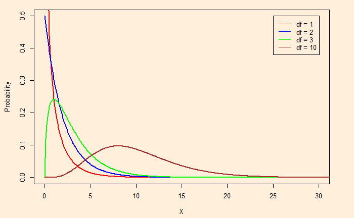
Chi-Square is a family of continuous distribution, widely used in hypothesis tests. The shape of a chi-square distribution is determined by what is known as the degree of freedom (df).

A chi-square test operates by comparing the observed distribution to what you expect if there is no relationship between the categorical variables.

Chi-Square Distribution Read More »

Likelihood Function – Part II

In the previous post, we estimated the likelihood of getting six people sick for two parameters (prevalence), 7% and 8%. We can also calculate the ratio between the two likelihoods:

L(theta = 0.07 | data = 6) / L(theta = 0.08 | data = 6) = 0.153 / 0.123 = 1.24. 

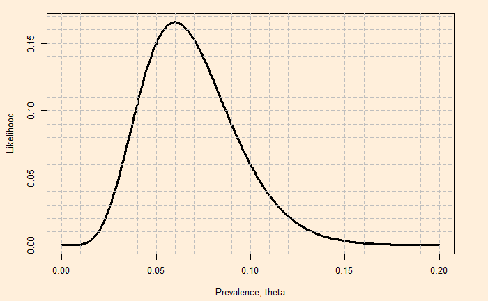
It means that the prevalence of 7% supports the data 1.24 times more than the prevalence of 8%. What about a sweep of likelihood over the entire parameter space? The function that gives the distribution of likelihoods of all possible values of parameters for a given data is the likelihood function.

As the parameter (theta) defines a model (e.g., binomial probability mass function), what the likelihood function is telling us is, given I have this data, what is the chance that the given model is true? In other words, we want the model that is mostly to have produced our data.

Likelihood Function – Part II Read More »

Likelihood Function

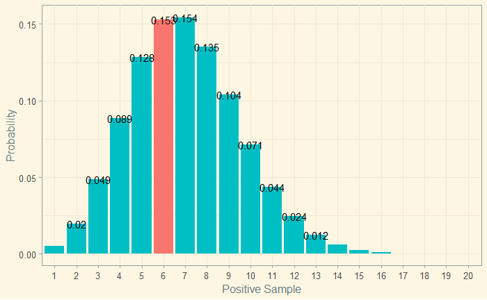
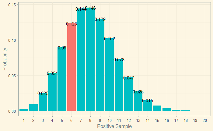
Consider two possible prevalence values for a rare disease, 0.07 and 0.08, respectively. If 100 samples from each city are taken, and six people are found positive, which prevalence value is likely?

Let’s visualise the situation 1:

And the situation 2:

It is clear that the first possibility, the prevalence (‘the parameter’) 0.07, is more likely, given 6 people tested positive as probability = 0.153 for the first case is > 0.123 for the second.

Summarising: for the parameter of 7%, the probability of getting six out of a hundred is 0.153. It becomes the likelihood.
L(theta = 0.07; y = 6) = 0.153 and L(theta = 0.08; y = 6) = 0.123

Here is the R code that generated the plot in situation 2.

xx <- seq(1,20)
P <-  dbinom(xx, 100, prob = 0.08)
binom_data <- data.frame(xx, P)

binom_data %>%  ggplot(aes(x=xx, y=P, label=P, fill=factor(ifelse(xx==6,"Highlighted","Normal")))) +
  geom_bar(stat="identity", show.legend = FALSE) +
  geom_text(aes(label=factor(ifelse(P > 0.01, round(P, 3),"")))) +
  scale_x_discrete(name = "Positive Sample", limits=factor(seq(1, 20, 1))) +
  scale_y_continuous(name = "Probability") +
  theme_solarized(light = TRUE) 

Likelihood Function Read More »

Likelihood Ratio – Fagan’s Nomogram

We have seen the likelihood ratio as the property of a diagnostic tool. Let’s take the fictitious screening tool we evaluated in the last post with LR+ = 10.7. Imagine a patient comes to a clinic with a few symptoms of a disease with a prevalence of 0.1 (very likely, age-adjusted), and this screening is a possible option. Would you recommend this? Note that the doctor will decide on further (costly) treatment only if she gets a conformation (posterior probability) of > 50% chance of the disease.

From the relationship we derived last time, 

OR_Post = LR x OR_Pri

Odds ratio (posterior) = 10.7 x 0.11 = 1.07
P(poterior) / (1 – P(poterior)) = 1.88
1/P(poterior) = 1 + 1/1.88
P(poterior) = 1.88/2.88 = 0.54

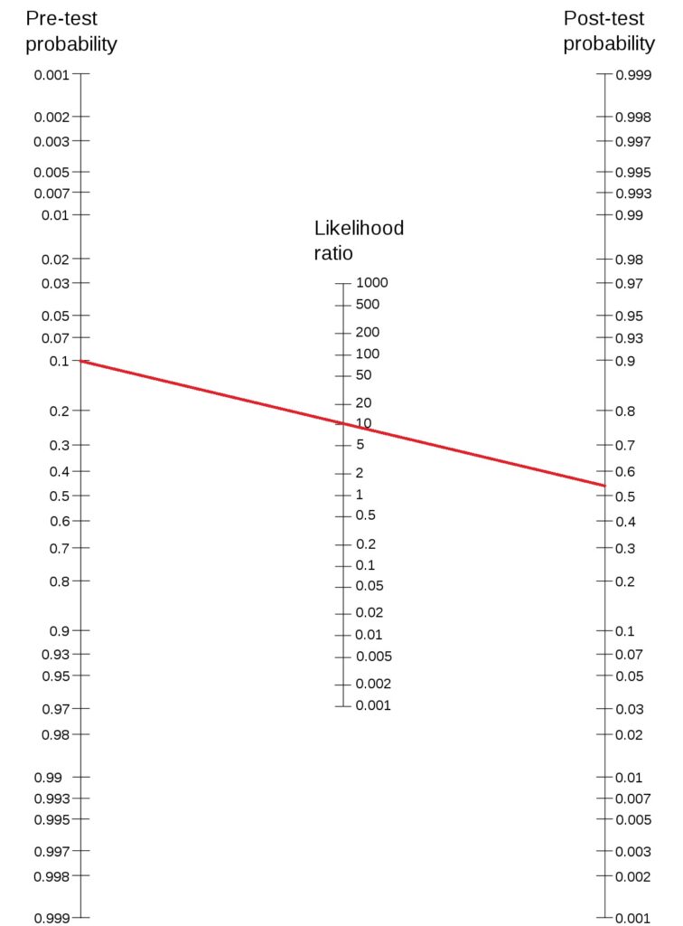
A nomogram of the following type is built to make such calculations simpler.

Draw a line from the ‘pre-test probability’ to ‘the likelihood ratio’ and extend it to the ‘post-test probability line. The intersection gives the posterior probability.

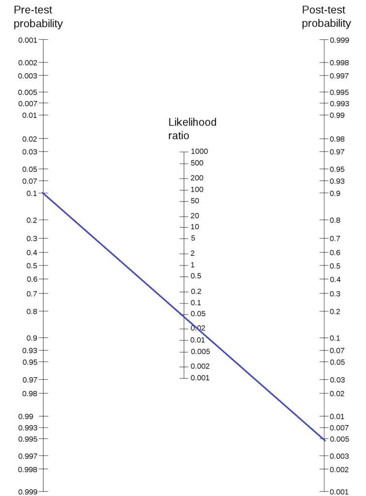
Here is an illustration of the method. Let’s use Fagan’s nomogram for the previous case,

To answer the original question: this test may be recommended as it can bring the probability over 0.5 if the test comes positive. Not to forget, if the test comes negative (LR- = 0.044), the posterior probability becomes 0.005.

Smaller prior

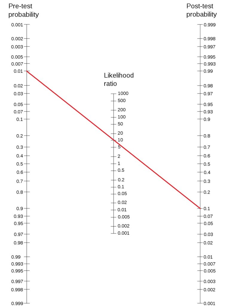
On the other hand, if the prior probability is lower, say, 0.01, as you can see below, the test is not very useful to make a conclusive decision.

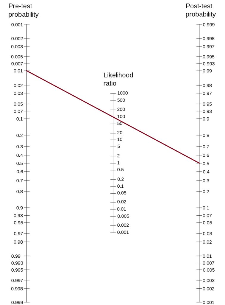
Such a disease would require a diagnostic tool with a likelihood ratio of 100 or above to make a decision. Connect 0.01 (prior probability) to 0.5 (minimum decision criterion) and find out the likelihood ratio.

Likelihood Ratio – Fagan’s Nomogram Read More »

Likelihood Ratio and Posterior Odds

We know how the updated (posterior) disease probability is related to the prevalence (prior) via Bayes’ relationship.

\text{Posterior} = \frac{Sensitivity *  Prior}{Sensitivity *  Prior + (1-Specificity)*(1- Prior)}

Here, the ‘posterior’ and ‘prior’ are probability values. The corresponding odds ratio may be calculated using the following formula,

\text{Odds Ratio} = \frac{P}{1-P}

Using this definition, we estimate the odds ratio of the posterior as:

\\ OR_{post}= \frac{Posterior}{1-Posterior} \\ \\ = \frac{\frac{Sensitivity *  Prior}{Sensitivity *  Prior + (1-Specificity)*(1- Prior)}}{1 - \frac{Sensitivity *  Prior}{Sensitivity *  Prior + (1-Specificity)*(1- Prior)}} \\ \\ = \frac{Sensitivity *  Prior} {(1-Specificity)*(1- Prior)} = \frac{Sensitivity} {(1-Specificity)}\frac{Prior}{(1- Prior)}}

Notice the two terms: the first term, Sensitivity / (1 – Specificity), is the likelihood ratio and the second term, Prior / (1-Prior), is the odds ratio of the prior. Therefore,

OR_Post = LR x OR_Pri

Example

A new diagnostic tool yielded the following results.

  • A total of 1,000 individuals took the test.
  • 435 individuals had positive results, and 565 were negative.
  • Out of the 435 positive, 381 of them had the disease.
  • Out of the 565 negative, 549 did not have the disease.

What is the positive likelihood ratio of the test method?

From the data, true positives (TP) are 381. Then 435 – 381 = 54 must be false positives (FP).
Similarly, the true negatives (TN) are 549. 565 – 549 = 16 must be false negatives (FN).

Sensitivity = TP/(TP + FN) = 381/(381+16) = 0.96
Specificity = TN/(TN+FP) = 549 / (549 + 54) = 0.91

The likelihood ratio, therefore, is,
0.96 / (1 – 0.91) = 10.7

Likelihood Ratio and Posterior Odds Read More »

Likelihood Ratio

The likelihood ratio is the proportion of people with a disease and a test result vs. people without the disease and the same test result. In other words,

P(+ve AND D) / P(+ve AND D-) = P(TP) / P(FP) = [TP/TP+FN] / [FP/FP+TN]
LR+= Sensitivity / 1 – Specificity.

This is the positive likelihood ratio (LR+)

In the same way, there is a negative likelihood ratio (LR-),
P(-ve AND D) / P(-ve AND D-) = P(FN) / P(TN) = TP/TP+FN
LR- = (1-Sensitivity) / Specificity

Note that both these ratios don’t depend on the prevalence of the disease but on the measurement techniques. A likelihood ratio of close to 1 means that the particular test has little influence on determining whether the patient has the suspected condition or not. Likelihood ratios > 10 and < 0.1 are considered to provide robust evidence for and against the diagnoses, respectively.

Likelihood Ratio Read More »

Climate Change – Pew Research Survey

Motivated reasoning is the tendency to favour conclusions we want to believe despite substantial evidence to the contrary. A famous example is climate change. In the US, for example, Democrats and Republicans disagree on the scientific consensus. A recent Pew Research survey on climate change presents the magnitude of this divide.

Prioritise alternative energy

At the highest level, 67% of people support this view, which is pretty impressive. But that is 90% Democrats (and Democrat-lining) and 42% Republicans (and leaning). The only silver lining is that 67% of Republicans under age 30 support alternative energy developments.

Climate change – a major threat to the well-being

Here again, the difference between the two parties is stark. In the last 13 years, the views from the Democrats have steadily increased from 61% to 78%, acknowledging climate change as a major threat. It has remained steady and low for the Republicans – at 25% in 2010 and 23% in 2022.
Interestingly, 81% of French and 73% of Germans regard it a threat.

Americans’ views of climate change: Pew

Climate Change – Pew Research Survey Read More »