Science

Genetic Drift

We have seen natural selection as one mechanism of evolution. To clarify the whole process, this way of evolution involves two steps: 1) a random (accidental) modification of genes (mutation), followed by 2) a proliferation of a certain kind because it somehow fits well with its environment (natural selection).

But natural selection is not the only mechanism for evolution. Another means of evolution is genetic drift. In such cases, there could be no features of the genetically different versions of the species that have advantages or disadvantages from the environment. Still, random fluctuation causes one of the gene types (allele) to reduce its frequency. This also suggests that this feature is especially significant in small, isolated populations.

To give a (silly) example to distinguish the two types of evolution, we have seen the story of A moth named Biston betularia earlier. The survival probability of the black-coloured moths was higher in the industrialised (coal-polluted!) England. This is an example of natural selection. Now, think about a small population of 20 moths – 15 white and five yellows in a bright, normal neighbourhood. Someone accidentally stepped over the group, perishing seven whites and all (5) yellows. We know neither species had a special trait to withstand the boots. Yet, in the end, only eight whites were the only survivors. They then increased to a large group of white moths.
Genetic Drift Read More »

Average Temperature in Jakarta

The average temperature in June in Jakarta is 32 oC with a standard deviation of 5 oC. If the temperature in June follows a normal distribution:

  1. What is the probability of observing higher than 40 oC on a random June day in Jakarta?
1 - pnorm(40, mean = 32, sd = 5)
0.0548

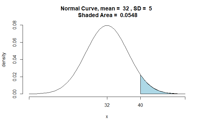
Let’s estimate the same thing using the ‘pnormGC’ of ‘tigerstats’ package.

pnormGC(40, mean = 32, region = "above", sd= 5, graph = TRUE)

2. How cold are the coldest 10% days in June in Jakarta?

 qnorm(0.10, mean = 32, sd = 5)
25.59224
 pnormGC(25.59224, mean = 32, region = "below", sd= 5, graph = TRUE)

Average Temperature in Jakarta Read More »

The Power Function 

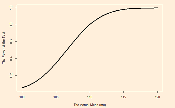
In the last post, we have seen the power of the hypothesis test for a mean, which is away from the null hypothesis. What happens if the true mean is further away, say 110 instead of 108? Let’s run the following code and you get it.

power_calc <- function(alt){

Null_mu <- 100
sigma <- 16
N_sample <- 16
alpha <- 0.05
Alt_mu <- alt

z <- qnorm(alpha, 0, 1, lower.tail = FALSE)
X_05 <- z * sigma /sqrt(N_sample) + Null_mu
Z_cum <- (X_05 - Alt_mu) / (sigma/sqrt(N_sample))
pnorm(Z_cum, 0, 1, lower.tail = FALSE)  

}

power_calc(110)

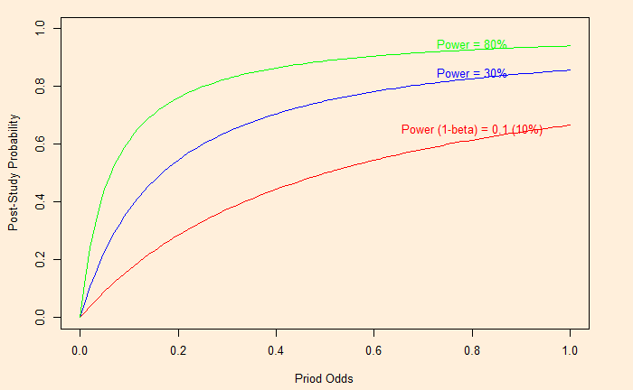
You see, the power is increased from 0.64 to 0.8. The whole spectrum of power values from the null hypothesis mean (100) all the way to 120 is shown below.

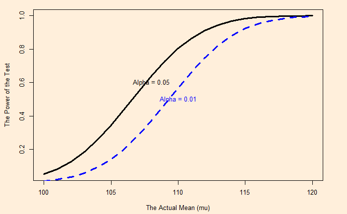
When alpha is reduced, the power is also reduced (type II error increases).

Reference

Power Functions: PennState

The Power Function  Read More »

IQ Power

Let’s assume the IQ of a population is normally distributed with a standard deviation of 16. A hypothesis test collected 16 samples for the null hypothesis of mean IQ = 100 for a significance level of 5%. What is the power of the hypothesis test if the true population mean is 108?

Definition: The power of a test is the probability that it will correctly reject the null hypothesis when the null hypothesis is false.

Step 1: Estimate the Z-score for the alpha (significance level)

qnorm(0.05, 0, 1, lower.tail = FALSE)
1.645

Step 2: Estimate IQ corresponds to Z = 1.645

\\ Z = \frac{\hat{X} - \mu}{\sigma/\sqrt{n}} \\ \\ \hat{X} = \frac{Z \sigma}{\sqrt{n}} + \mu

1.645 * 16 / sqrt(16) + 100 =  106.58

Above the IQ average of 106.58, the Null hypothesis (that the mean = 100) will be rejected.

Step 3: Estimate Z-score at X = 106.58 for mean = 108

Z = \frac{106.58 - 108}{16/\sqrt{16}} = -0.355

The entire area above Z = -0.355 is included in the power region (the area below Z = -0.355 will be the false negative part as the null hypothesis will not be rejected).

Step 4: Estimate the cumulative probability > Z = -0.355

pnorm(-0.355, 0, 1, lower.tail = FALSE)
 0.639

The power is 0.639 or 64%

Reference

Power Functions: PennState

IQ Power Read More »

Type I, Type II and pnormGC!

Alan knows the average fuel bill of families in his town last year was $260, which followed a normal distribution with a standard deviation of $50. He estimated this year’s value to be $278.3 by sampling 20 people. He then rejected last year’s average (the null hypothesis) in favour of an alternate of average > $260.

1. What is the probability that he wrongly rejected the Null hypothesis?

The probability is estimated by transforming the normal distribution with mean = 260 and standard deviation = 50 to a standard normal distribution (Z):

The ‘pnormGC’ function of the ‘tigerstats’ package makes it easy to depict the distribution and the region of importance.

library(tigerstats)

sample <- 20
null_mean <- 260
ssd <- 50
data <- 278.3

zz <- round((data - null_mean)/(ssd/sqrt(sample)), 2)
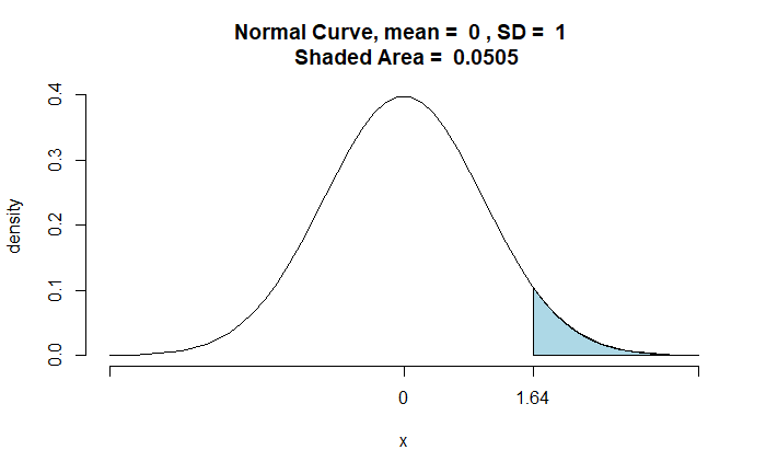
pnormGC(zz, region="above", mean=0, sd=1, graph=TRUE)

The probability of incorrectly rejecting the null hypothesis is 0.0505 (5.05%). It is the probability of Alan committing a Type I error.

If Alan accepts a 5% Type I error, he will reject the null hypothesis for every value > 278.3 and accept all values < 278.3.

2. If so, what is the probability of wrongly rejecting the alternate hypothesis that the true population mean for this year = $290?

sample <- 20
alt_mean <- 290
ssd <- 50
data <- 278.3

zz1 <- round((data - alt_mean)/(ssd/sqrt(sample)), 2)
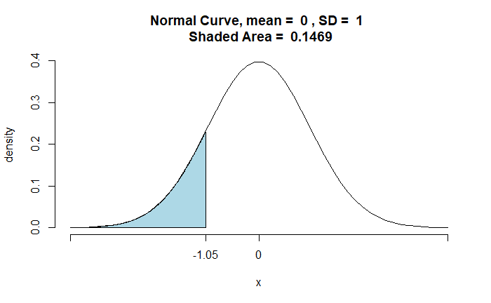
pnormGC(zz1, region="below", mean=0, sd=1, graph=TRUE)

The shaded area represents all the values < 278.3. And it is the probability of Type II error.

Type I, Type II and pnormGC! Read More »

Reproducibility and Replicability

If I were to define science in one phrase, it would be ‘hypothesis testing’. In the report published in 2019, the committee appointed by the Science Foundation (NSF) defined two fundamental terms connected to scientific research (and hypothesis testing): reproducibility and replicability.

Reproducibility

Reproducibility is about computation. It is about consistent calculation output from the same input data, computational steps, methods, codes, etc.

Replicability

Replicability involves new data collection using methods similar to those employed by previous studies.

References

National Academies of Sciences, Engineering, and Medicine 2019. “Reproducibility and Replicability in Science“. Washington, DC: The National Academies Press. https://doi.org/10.17226/25303.

Reproducibility and Replicability Read More »

Three Recommendations on the p-Value Threshold

In the previous post, we saw the problem of indiscriminately using the threshold p-value of 0.05 to test significance. Benjamin and Berger, in their 2019 publication in The American Statistician, urge the scientific community to be more transparent and make three recommendations to manage such situations.

Recommendation 1: Reduce alpha from 5% to 0.5%

It is probably a pragmatic solution for people using p-value-based null hypothesis testing. We know 0.005 corresponds to a Bayes Factor of ca. 25, which can produce good posterior odds for prior odds as low as 1:10. But what happens if the prior odds are lower than 1:10 (say, 1:100 or 1:1000)?

Recommendation 2: Report Bayes Factor

Bayes factor gives a different perspective on the validity of the alternative hypothesis (finding) against the null hypothesis (default). Once it is reported, the readers will have a feel of the strength of the discovery.

Bayes Factor (BF10)Interpretation
> 100Decisive evidence for H1
10 – 100Strong evidence for H1
3.2 – 10Substantial evidence for H1
1 – 3.2No real evidence for H1

Recommendation 3: Report Prior and Posterior Odds

The best service to the community is when researchers estimate (and report) the prior odds for the discovery and how the evidence has transformed them to the posterior.

Reference

[1] Benjamin, D. J.; Berger, J. O., “Three Recommendations for Improving the Use of p-Values”, The American Statistician, 73:sup1, 186-191, DOI: 10.1080/00031305.2018.1543135

[2] Kass, R. E.; Raftery, A. E., Bayes Factors, Journal of the American Statistical Association, 1995, 90(43), 773

Three Recommendations on the p-Value Threshold Read More »

Bayes Factor and p-Value Threshold

Blind faith in p-value at 5% significance (p = 0.05) has contributed to a lack of credibility in the scientific community. It has affected the class, ‘discoveries’ more than anything else. Although the choice of threshold p-value = 0.05 was arbitrary, it has become a benchmark for studies in several fields.

It is easier to appreciate the issue once you understand the Bayes factor concept. We have established the relationship between the prior and posterior odds (of discovery) in an earlier post:
Posterior Odds = BF10 x Prior Odds

Studies show that the prior odds of typical psychological studies are 1:10 (H1 relative to H0). For clarity, H1 represents the hypothesis leading to a finding, and H0 is the null hypothesis. In such a context, a p-value, which is equivalent to a Bayes factor of ca. 3.4, makes the following transformation.

Posterior Odds = 3.4 x (1/10) = 0.34 ~ (1/3); the odds are still in favour of the null hypothesis.

On the other hand, if the threshold p is 0.005 (equivalent to a BF = 26),
Posterior Odds = 26 x (1/10) = 2.6 (2.6/1); more in favour of the discovery.

Reference

Redefine statistical significance: Nature human behaviour

Bayes Factor and p-Value Threshold Read More »

Bayes Factor and Rare Diseases

Let’s revisit Sophie and the equation of life (a.k.a. Bayes’ theorem). We know that the chance of breast cancer became about 12%, starting from a state of no symptoms and a positive test result. That too from a test that has 95% sensitivity and 90% specificity. And the secret behind this mysterious result was the low prevalence or prior probability of the disease.

P(D|TP) = P(TP|D) x P(D) /[P(TP|D) x P(D) + P(TP|!D) x P(!D)]

Here, TP represents test positive, D denotes disease and !D is no disease.

Rare disease

How do you describe a rare disease? As a simple approximation, let’s define it as an illness with a chance of 1% or lower to occur. We’ll now apply the Bayes’ rule for a few cases of P(D) (0.01, 0.005, 0.001, etc) and see how the probability updates when the test comes positive.

P(D)
Prior
P(D|TP)
Posterior
Posterior
/ Prior
(ratio)
0.010.0888.8
0.0050.0469.2
0.0010.00949.4

Can you estimate the Bayes factor for the above case?

Bayes FactorD-!D = P(TP|D) / P(TP|!D)
P(TP|D) = sensitivity = 0.95
P(TP|!D) = 1 – specificity = 1 – 0.9 = 0.1
BFD-!D = 0.95 / 0.1 = 9.5

As a heuristic, for rare diseases, the updated chance of having the disease post a positive diagnostics equals Bayes factor x prevalence.

Bayes Factor and Rare Diseases Read More »