Life

Does Bayes’ Approach Mimic The Natural Learning Process?

We have seen Bayes’ theorem before. It is a way of updating the chance of an event to occur based on what is known as a prior probability. Check the formula, in case you forgot it because we will use it again.

We do an exercise to illustrate today’s storyline, courtesy – a course in Bayesian statistics run by the University of Canterbury. You learn about a café in town. The shop has two baristas, one experienced and one less experienced. You also came to know that the experienced makes excellent coffee 80% of the time, good coffee 15% and average coffee 5% of the time. For the less experienced, the performance stats are 20%, 50% and 30%, respectively. Your task is to go to the cafe, order, enjoy the coffee and identify the barista.

cafe gourmande, french, café-258201.jpg

You order a cup of coffee and find it an excellent one. Is this prepared by A? Let’s use Bayes’ equation. But, where do you start? You need a prior probability to begin. One way is to assign a 50-50 chance of encountering A on that day. Another way is to use your knowledge about the workdays per week, which sounds better than 50-50.

The chance that A made your coffee, given that it was an excellent coffee:
P(A|E) = 0.8 x (5/7) / [0.8 x (5/7) + 0.2 x (2/7)] = 0.90

There is a 90% chance that A prepared your coffee. In other words, the initial estimate of (5/7), based on the work pattern, is updated to a higher value.

You got time to spend on another cup of coffee, and it turned out to be an average one! Now you update your estimate using the following calculation,
= 0.05 x (0.9) / [0.05 x (0.9) + 0.3 x (0.1)] = 0.625

Note that the new prior probability is 0.9 and not 5/7. The updated chance (also known as the posterior probability) is still in favour of A but reduced from 90% to 63%.

The true scientist in you tries another coffee, and the outcome was an excellent coffee, and the updated chance is now 87%. At this stage, you decided to end the exercise and conclude that the barista of that day was the experienced one.

Natural Learning Process

This process of updating knowledge based on new information is considered by many as natural learning. I would view this as the ideal learning process, which rarely happens, naturally. In real life, most of us like to carry on the baggage of knowledge – be it from our parents, peers or other dogmatic texts, and resists every opportunity to update. In other words, you ignore new information or the information that does not tally with the existing.

In my opinion, scientific training is the only way to counter the tendency to carry on the baggage. The evidence-based worldview is not natural and needs forceful cultivation.

Back to Café

In the barista story, you may be wondering why the process repeated a few times, and the enquirer settled for a lower probability than what occurred after the first cup. To get the answer, consider the exact three cups of coffee but in a different order, say the average one first. What difference do you see?

Does Bayes’ Approach Mimic The Natural Learning Process? Read More »
The Claim Instinct and One-Child Policy

The blame instinct drives us to attribute more power and influence to individuals than they deserve, for bad or good. Political leaders and CEOs in particular often claim they are more powerful than they are.

Hans Rosling from the book Factfulness

Blame instinct and claim instinct! For a modern-day leader, be it a politician or a CEO, the former brings the power, and the latter keeps it. In one of the previous posts, we have looked at the unsubstantiated blame against Muslims in India and the reality of population growth. This time we look at the other side, the claim factories and the success of child-control policies.

Most of you are familiar with the one-child policy of China and the ‘blockbuster’ success that it brought. I remember this message used to echo everywhere when I was growing up in the eighties. Interestingly, even today, after all these years, when so much data are publically available for free that rejected the whole notion, some leaders maintain the rhetoric.

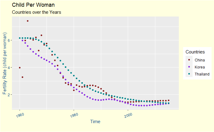
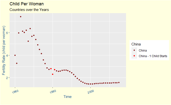
Come back to the China report. The following is a plot of the fertility rate of women in China from 1960 to 2016. For complete data and visualisations, go to the gapminder website.

As per Wikipedia, the Chinese government started the policy in 1980. In the plot, I’ve marked three years – 1979, 1980 and 1981 – in red to show, in the big picture, the timing when the government was implementing the policy. The Chinese women fertility rates have been on a sliding-down path since the 70s. The policy of 1980 may have only reduced its pace, but that I leave to your imagination.

My claim above based on a plot is not entirely bulletproof. It is impossible to show that the policy did not work as the child per woman was either kept low or decreased during the period. To discover the results and remove any anomalies, we must compare the trend with other countries. So, let’s examine two countries in East Asia that did not impose such a burden on their people – South Korea and Thailand.

Did it stop in South Korea and Thailand? No, the whole of Asia has shown declines in female fertility since the middle of the twentieth century.

Thoughtful Examinations of Data

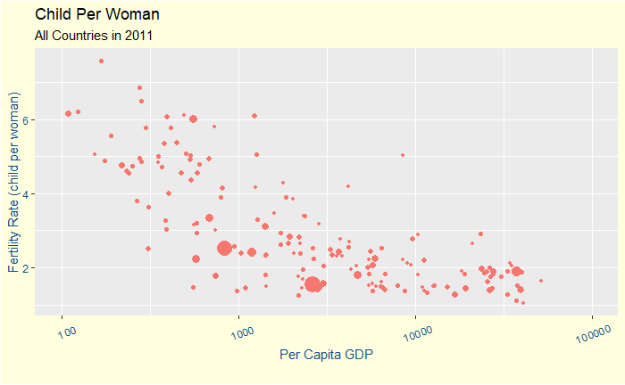
The results show the power of evidence and reflect the time we are living, the age of free and publically available data. The data showed beyond doubt that economic status and education are stronger predictors of smaller families than other popular beliefs, such as religion or strong rulers.

The size of the symbol represents the population of the country.

In simple words, when a mother is educated and financially independent enough to know that her society has the means to get her children to pass their childhood, she starts to prefer a smaller family! A family that can have a quality life and where the children can climb the social and economic ladder.

Why are Claims So Powerful?

It is so convenient. Something that happened without any intervention from the all-powerful is difficult for humans to admit, especially for the powerful humans! The public also believes them as the claims go hand in hand with the almighty image of the powerful.

Data used for Post is from gapminder

The Claim Instinct and One-Child Policy Read More »

The population of South Asia

Mixing is the reality of life; pure only exists in our imagination.

Humans have this love for purity and feel shame about the undeniable reality of mixing. While people in some parts of the world are proud of eating a ‘purely’ vegetarian diet, others list everything they could recollect from their harddisks to proclaim their superior ancestry. They are all right, but only for a negligibly short duration in history. Human history does not give a damn about vegetable eaters, and the same for any exclusive ancestry!

A landmark research paper came out in September 2019 in the journal Science titled, ‘The formation of human populations in South and Central Asia’. It was a report based on ancient DNA data from 523 individuals spanning the last 8000 years, from Central Asia and northernmost South Asia.

Migration of Yamnaya Steppe Pastoralists

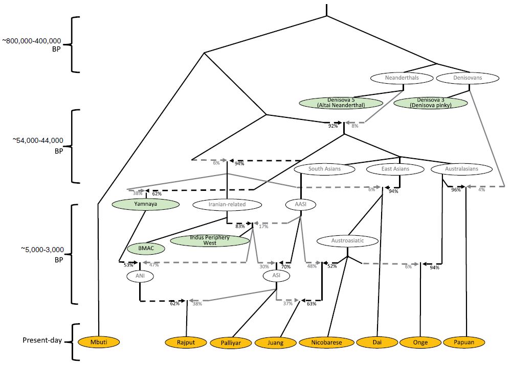
The paper was primarily on the migration of the Eurasian Steppe to South Asia around 3000 years ago. The ‘Steppe Ancentry’ or Yamnaya culture was active around 5000 years ago in present-day Ukraine and Russia. The folks from that region had travelled to either side of the world, to Europe and South Asia. Today we talk about the guys and, perhaps some girls, who migrated to the east.

It is relevant here to talk about another DNA study published in Nature in 2009. This study genotyped 125 DNA samples of 25 different groups of India and did what is known as a Principal Component Analysis (PCA) of the data. Based on the similarities of the allele, they found a relationship between people of the North and South of India. An ancestral component, they call it ANI (Ancestral North Indian), varied from 76% for the North to 40% in the south. The remaining fraction is the ASI (Ancestral South Indians). Note that a ‘Pure’ ASI, closer to the earliest humans (travelled from Africa, of course), was not seen in that study.

Where are those people? That is next

Flashback

ASI was ‘ruling the land’ and Indus Valley Civilisation (IVC) was flourishing when the Steppe folks arrived in present-day India. But that would change soon, and the visitors would form a mix, which is the base of the continuous band from North to South that we saw earlier. So was ASI was the original one? The answer is a firm NO. ASI was a mix of what is known as AASI and a group of people with Iranian farmer ancestry. And who were this AASI? Well, they were the people who came 40,000 years ago, yes, from the cradle of homo sapiens, Africa. Of course, the Iranian farmers also went from Africa, but a few tens of thousands of years earlier.

Piecing All Together

The following picture, copied from the Science paper, summarises the whole story.

Why Is It Important?

It is always fun to learn more and more about the incredible spread of homo sapiens from Africa to the rest of the world. It is equally wonderful to note how dynamic was the intermixing of population. Also, notice one irony. These results, the vivid stratification of ANI and ASI, were possible due to their obsession with endogamy in the last few hundred years. That way, they preserved the signatures of the founders or else it would have been a complete mixing of genes.

The formation of human populations in South and Central Asia: Science

Reconstructing Indian population history: Nature

The population of South Asia Read More »

Probabilities and Evolution

What is the probability of creating a fully developed animal or a human being? Creationists often use this argument to challenge science, but that is understandable. What is depressing is to see many scientists, too, falling into their trap.

Look at this mind-boggling probability. Think about one biological molecule in our body – haemoglobin. The molecule consists of 4 chains of amino acids, and each chain is about 146 links consisting of a possible 20 amino acids. So, to get a functional molecule, it needs to get one right out of (20)146 options. How is it then possible to have the whole human body created? Since your random processes can’t explain such ‘beautiful crafts’ of nature, you better accept my design theory!

It is a valid question, except that today’s complex systems are not formed like this. The answer lies in evolution. You and I are today because of the accumulated small changes. Not from any single change. Getting a small change is relatively easy, with about a few million unforced errors happening every day.

The complex systems we see today all originated from simpler systems. And those simpler ones, from even simpler ancestors. Until the stage, when the first life, some RNA-based self-replicating molecule, was formed! And how are they made? By chance in the chemistry laboratory of the earth using simple gases in the presence of heating, cooling and lightning. Stanley Lloyd Miller and Harold Clayton Urey proved that in 1953 by using methane, ammonia, water, hydrogen, and electric discharge to produce amino acids. Subsequent works of scientists synthesised the building bases of RNA from simple molecules.

In my post on SLC24A5 or the one on plant breeding, we have seen that a simple change in a random gene location can produce wonders. Think about it. There have been 3.5 billion years passed since the first life. Millions of trivial changes happened, a few of them passed through the sieves of nature, and a number of them got rejected to extinction. It is called natural selection.

Richard Dawkins: The Blind Watchmaker

Blind Watch Maker

Stanley L Miller, A production of Amino Acids Under Possible Primitive Earth Conditions, Science, 1953

Formation of nucleobases in a Miller–Urey reducing atmosphere, PNAS, 2017

Probabilities and Evolution Read More »

T&K Stories – 4. Anchoring and Its Impact on Our Decisions

This time we discuss another story from the paper of Tversky and Kahneman – about the biases originating from our inability to make adjustments from an initial value. In other words, the initial value anchors to our head.

To illustrate this bias: the following expressions were given to two groups of high-school students to estimate in 5 seconds.
to the first group: 1 x 2 x 3 x 4 x 5 x 6 x 7 x 8
to the second group: 8 x 7 x 6 x 5 x 4 x 3 x 2 x 1

The median estimate for the first group was 512, and that of the second was 2250 (the correct answer is 40320)!

Our Estimation of Success and Risks

Overestimation of benefits and underestimation of downsides are things we see every day. On the one hand, it was necessary for us, as a species, to make progress, yet it could seriously land in failure to deliver quality products in the end.

Conjunctive Events

Imagine, the success of a project depends on eight independent chances, each with 95% probability (almost a pass for each!). So overall, the project has (0.95)8 = 66% chance of success. Often people overestimate this as the number 0.95 gets them into a belief of surety of success. These are conjunctive events, where the outcome is a joint probability or conjunction with one other.

Disjunctive Events

A classic case of a disjunctive event is the estimation of risk. Each stage of your project has a tiny probability, about 5%, that can stop the business. What is the overall risk of failing? You know by now that you can’t multiply all those tiny numbers, instead estimate the chance not to lose in any step and then subtract it from 1. (1 – (0.95)8) = 33%. You don’t finish in one out of three cases. People underestimate risks because the starting point appears too small to be significant.

Tversky, A.; Kahneman, D., Science, 1974 (185), Issue 4157, 1124-1131

T&K Stories – 4. Anchoring and Its Impact on Our Decisions Read More »

T&K Stories – 3. Biases of Imaginability

Consider a group of 10 people who form committees of k members, 2 < k < 8. How many different committees of k members can be formed?

Judgment under Uncertainty: Heuristics and Biases, Tversky and Kahneman

The third story from Tversky and Kahneman paper is about the role of imaginability in the estimation of probabilities. Consider this group of 10 people who form committees of a minimum of 2 up to a maximum of 8. To find how many possible ways to form teams, you need to apply what is known as Combinations, which is nothing but the binomial coefficient that you have seen earlier. i. e. Combinations of n things taken k at a time without repetition.

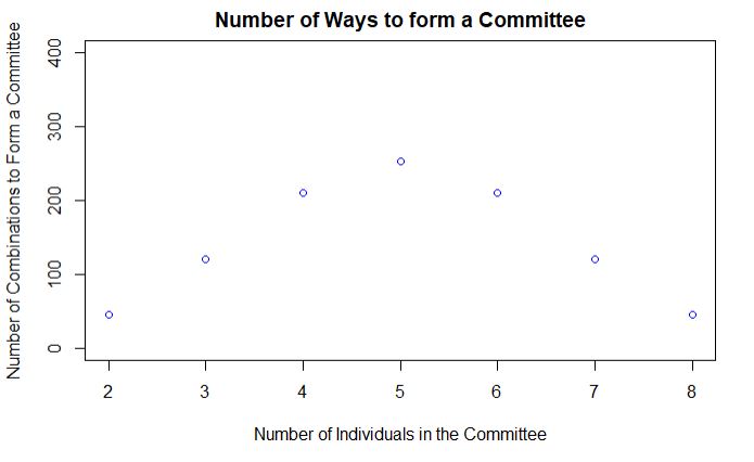
For 3-member teams, it comes out to be 10C3 or 120. The choice increases to the maximum for 5 (252 combinations), and then decreases symmetrically such that nCk = nCn-k (number of 3-member groups = number of 7-member groups and so on).

The following R code uses the function choose(n,k) to evaluate the binomial coefficient and plots the outcome.

committe <- function(n,k){
  choose(n,k)  
}

diff <- seq(2,8)
diff_com <- mapply(committe, diff, n = 10)

plot(x = diff, y = diff_com, main = paste("Number of Ways to form a Committee"), xlab = "Number of Individuals in the Committee", ylab = "Number of Combinations to Form a Committee", col = "blue", ylim = c(0,400))

It requires number crunching, and mental constructs don’t always help. In a study, when people were asked to make guesses, the median estimate of the number of 2-member committees was around 70; 8-member committees were at 20. So, imagining a few two-member teams were possible in mind, whereas 8-member groups were beyond its capacity.

Tversky, A.; Kahneman, D., Science, 1974 (185), Issue 4157, 1124-1131

T&K Stories – 3. Biases of Imaginability Read More »

T&K Stories – 2. Birth of Baby Boys

A certain town is served by two hospitals. In the larger hospital about 45 babies are born each day, and in the smaller hospital about 15 babies are born each day. As you know, about 50 percent of all babies are boys. However, the exact percentage varies from day to day. Sometimes it may be higher than 50 percent, sometimes lower.

For a period of 1 year, each hospital recorded the days on which more than 60 percent of the babies born were boys. Which hospital do you think recorded more such days?

b The larger hospital
b The smaller hospital
b About the same

Judgment under Uncertainty: Heuristics and Biases, Tversky and Kahneman

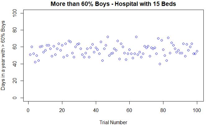
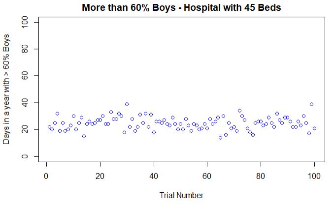
If you recall the law of large numbers, you would have guessed the correct answer, i. e. the smaller hospital. Because as the number of births increases, the gender of the baby comes closer to the expected percentage of 50.

If you still doubt, let’s run a simple Monte Carlo run using the following R code,

days  <- 365
birth <- 15
boy   <- 0.5
boys  <- replicate(days, {
  prob_birth <- sample(c(0,1), birth, prob = c((1-boy), boy), replace = TRUE)
  mean(prob_birth)*100
})

sum(boys > 60)

Run this code 100 times and plot the answers, the probabilities of a day in which more than 60% were boys:

Now, change the number of births to 45 and re-run the calculations:

What about more than 60% of girls?

Let me end this piece with this one. Which hospital do you expect more number of days with less than 40% of boys? No marks for guessing: it is still the small hospital.

Tversky, A.; Kahneman, D., Science, 1974 (185), Issue 4157, 1124-1131

T&K Stories – 2. Birth of Baby Boys Read More »

T&K Stories – 1. Librarian vs Farmer

“Steve is very shy and withdrawn, invariably helpful, but with little interest in people, or in the world of reality. A meek and tidy soul, he has a need for order and structure, and a passion for detail.”

Judgment under Uncertainty: Heuristics and Biases, Tversky and Kahneman

Following the clues above, your task is to guess if Steve is a farmer or a librarian.

A significant proportion of people may have guessed Steve was a librarian. Some of the others who chose farmer may have done it so out of suspicion of the build-up. 

Back to Bayes’ics 

Remember the Bayes’ theorem? If not, read my earlier post, The Equation of life.  

P(Lib|D) = P(D|Lib) x P(Lib) / [P(D|Lib) x P(Lib) + P(D|noLib) x P(noLib)]

Let us check the chance for the frequent answer – that Steve was a librarian – to be true (P(Lib|D)). I am ready to support the argument that all librarians fit this stereotype (P(D|Lib) = 1) if that was a concern. It is unlikely to be valid, but I give you that benefit of the doubt. Estimating the prior probability of librarian in a set of farmers and librarians (P(Lib)) is the task that needs data. Based on the available data in the public domain, in the US, that ratio is 0.026!

P(D|noLib) or the description fitting farmers is tricky, but I make an assumption least 10% of the farmer community can have shy and withdrawn men! P(noLib) is nothing but 1 – P(Lib). Substitute all the numbers

(1 * 0.026)/[(1 * 0.026)+(0.1 * 0.974)] = 0.21.

Even if all the librarians fit your mental stereotype, you are right only 20% of the time. To paraphrase what late Hans Rosling used to say: a chimp would do a better job; she picks the correct answer 50% of the time.

It’s not about Maths

The message here is not about the math, nor about the research required to get an accurate answer. It is only about being mindful about our biases and how much they can lead to inaccurate perceptions about others.

References

Tversky, A.; Kahneman, D., Science, 1974 (185), Issue 4157, 1124-1131

Librarians in the US

Professional Workforce in the US

Statistics farmers in the US

T&K Stories – 1. Librarian vs Farmer Read More »

Tversky and Kahneman – and the Paper that Challenged Our Judgements

Let me talk about an article that I want you to read. It is titled ‘Judgment under Uncertainty: Heuristics and Biases‘, published in Science 1974. The paper is about heuristics, the mental shortcuts to arrive at decisions, and its inherent problems in real life. And the consequence? Implicit biases to gambling-addiction, stereotyping to micro-inequities.

We have seen in the past few posts how unreliable our intuitions about conditional probabilities can be. The authors give many stories to expose the errors in judgements that we are carrying.

I will go through their stories one by one in the coming days, but first, you read the paper.

Tversky, A.; Kahneman, D., Science, 1974 (185), Issue 4157, 1124-1131

Tversky and Kahneman – and the Paper that Challenged Our Judgements Read More »

The risk from the New Variant

As calamities from another variant of Covid19 is looming large, the omicron, be prepared for more confusing news in the coming days. It is also the right time to introduce the word risk. Risk has a specific technical meaning. It is the product of the likelihood of something to happen and the consequence.

Risk = likelihood x consequence.

Compare the delta variant with ones that came earlier. From the data, anecdotal evidence by individuals and evolutionary arguments, it became the public narrative that the consequence of infection with delta was similar to, or even mildly less dangerous. Did it mean the same for the risk? We can’t say until we know the likelihood. Delta turned out to be more than double as contagious as earlier ones. So the overall risk was much more than the first.

The second common argument was the case fatality rate. The CFR, as it is commonly known, was not high, they argued, but forgetting that almost a third of humanity was going to get it. A small fraction of a large number is still sizeable.

Black Swan Event

An extreme example of risk is the black swan event – a concept introduced by Nassim Nicholas Taleb through his book that carried the same name. These are unpredictable events and has infinite consequences.

Was the Covid pandemic a black swan event? As per the author himself, it was not a black swan event. People had predicted viruses attacks like these, and there were, however hypothetical, opportunities to control the disease at its onset, had there been a few steps taken by the originating country – be it intervention at the start or by just being more transparent.

But September 11 was one of them. It was never anticipated, and the consequence was enormous and far-reaching.

Delta variant

Black Swan Theory

Covid19 and Black Swan

The risk from the New Variant Read More »