Life

The Sailor’s Child problem

A sailor sails between two ports. At each port, he stays with a woman, both of whom want to have a child with him. The sailor is initially reluctant but changes his mind and tosses a coin to decide: if it’s a head, he will have a child with one and if it’s tail, with both. If heads come up, he will open up The Sailor’s Guide to Ports, and whichever port, out of the two, features earlier, he will choose the woman on that port.

If A is the son of the sailor, what is the probability that he is an only son?

We’ll go to the Bayes’ to find out the answer.

\\ P(O|C) = \frac{P(C|O) * P(O)}{P(C|O) * P(O) + P(C|NO) * P(NO)} \\ \\ P(O|C) = \frac{(1/2) * (1/2)}{(1/2) * (1/2) + 1 *(1/2)} = \frac{1}{3}

The Sailor’s Child problem Read More »

Car with No Rear View

Imagine you get a chance to buy a coffee shop. Here is what the owner tells you.
The current sales = $ 74,000 /yr
Shop rent = $30,000 /yr
Employee salary = $25,000 /yr
Coffee beans = $15,000 /yr
The cost of furniture and coffee machine = $45,000

How much are you willing to pay?

Market value

A simple valuation shows the shop can generate $4,000 a year (74,000 – 30,000 – 25,000 – 15,000) after paying for the rent, salaries and the purchase of the coffee beans. If you feel the shop will generate the same forever, you can do a simple (perpetuity) formula of 4000 / 0.1 = 40,000; 0.1 represents the discount rate of 10%. So you are willing to pay a maximum of $40,000.

The owner reminds you that she spent 45,000 just a few weeks ago to renovate. Will you change your mind? Sadly, it shouldn’t. The cost the owner sunk in the past can’t change the value it generates in the future. The buyer politely replies that she could get $500 more ($4,500) every year if she invested that 45,000 in the market at a 10% return. So what the owner spent (the book value) is immaterial to the buyer who calculated the market value.

Movie or football

Mat bought a ticket for a movie by paying $25. Just before he starts, he gets a phone call from John, who invites him to watch a football match. Mat likes football and John’s company, yet declines the invite because he has already spent the ticket price of the movie.

The money Mat spent is sunk, and what matters now is what gives him a good time (movie vs football with friends). But Mat falls for the sunk cost fallacy, the bad feeling for the loss on things that have already been spent against a better return in the future.

The concord of failures

The fallacy of sunk cost is common in big projects. Companies often hesitate to shut down projects midway when even they realise that it’s getting expensive and the product won’t make any economic benefit. They rationalise they invested too much to quit.

Social scientists hypothesise three reasons for this fallacy

  1. The loss aversion
  2. Desire not to appear wasteful
  3. To force one to do things that otherwise won’t happen

Psychology of decision making

The sunk cost fallacy is a powerful force that impacts decision-making. The issue with sunk costs is that they are the things of the past, but we pay too much attention to them. It’s the same feeling that keeps you attending the whole show of a terrible movie, eating everything ordered even when you are full, or continuing a nonfunctional relationship solely because the couple spent four years of their life together.

Reference

Sunk Costs: The Big Misconception About Most Investments: Sprouts

Car with No Rear View Read More »

Confounding vs Effect Modification

We have seen confounders before; it is a factor that associates with both exposure and outcome, thereby deceiving investigators of a causal relationship between the two.

For example, smoking is a confounder that misleads people to conclude that drinking can lead to lung cancer. In reality, smokers have a higher tendency to drink, and smokers have a higher tendency to get lung cancer. Until you stratify and find the impact of drinking on smokers and non-smokers, you are unlikely to figure out the error.

On the other hand, if the variable impact the outcome and not the exposure, it is an effect modification. A simple example is the immunisation status of an individual can impact the person’s susceptibility to getting the infection from the virus.

Confounding vs Effect Modification Read More »

Collider Bias – The Math

So far, I have addressed the collider-bias phenomena qualitatively. This time, I will try to show through numbers. It can be complex as the illustration involves a lot of arithmetic. The reference material provided at the end is a good read, further grasping the concept.

Imagine a situation where exposure is obesity, the risk factor is smoking, the outcome is mortality, and the collider is diabetes. If you are confused about what each represents, here is the expected storyline: A research group does study the impact of obesity on mortality in a set of people who have diabetes and comes up with a counterintuitive conclusion (perhaps that obesity decreases mortality)!

Set of information

Total study population = 1000
Smokers = 500
Non-smokers = 500
Obese = 500
Non-obese = 500
Baseline diabetes risk (non-smoking, non-obese)= 4%
Obesity increases diabetes risk by 16 % points
Smoking increases diabetes risk by 12% points
Baseline mortality risk (non-smoking, non-obese, nondiabetic)= 5%
Obesity increases mortality risk by 2.5% points
Smoking increases mortality risk by 15% points
Diabetic increases mortality by 5%

Calculations on the total sample

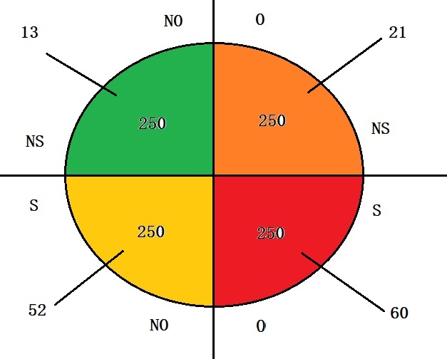
The overall study population is depicted as

Now, calculate the mortality rates of each quadrant and portion into obesity and non-obesity conditions.

Total mortality of NS-NO (non-smoking, non-obese) quadrant
= # of diabetic x diabetic mortality + # non-diabetic x baseline mortality
= 0.04 x 250 x (0.05 + 0.05) + (250 – 0.04 x 250) x 0.05
= 1 + 12 = 13
(note that diabetic mortality = baseline mortality + diabetic increases mortality)

S-NO (smoking, non-obese) quadrant
= # of diabetic x (diabetic mortality + smoking mortality) + # non-diabetic x (Baseline mortality + smoking mortality)
= (0.04 + 0.12) x 250 x (0.05 + 0.05 + 0.15) + (250 – (0.04 + 0.12) x 250) x (0.05 + 0.15)
= 52

S-O (smoking, obese) quadrant
= (0.04 + 0.12 + 0.16) x 250 x (0.05 + 0.05 + 0.15 + 0.025) + (250 – (0.04 + 0.12 + 0.16) x 250) x (0.05 + 0.15 + 0.025)
= 60

NS-O (non-smoking, obese) quadrant
= (0.04 + 0.16) x 250 x (0.05 + 0.05 + 0.025) + (250 – (0.04 + 0.16) x 250) x (0.05 + 0.025)
= 21

Calculations (for the total sample)
Mortality rate with obesity = (60 + 21) / 500 = 16.5%
Mortality rate without obesity = (13 + 52) / 500 = 13%
An increase of 3.5%

Calculations on the sub-sample

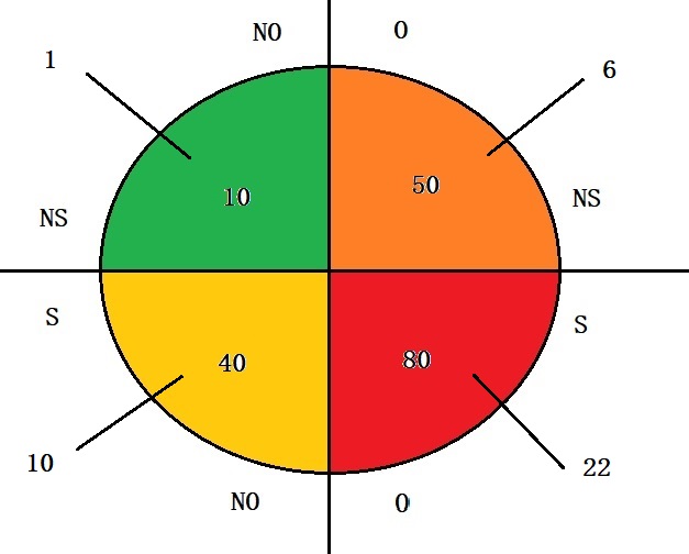
Suppose the study stratified the sample and analysed only people who have diabetes. The study sample space is as follows.

Do the same exercise as before

NS-NO quadrant
= # of diabetic x diabetic mortality
= 0.04 x 250 x (0.05 + 0.05)
= 1

S-NO quadrant
= # of diabetic x (diabetic mortality + smoking mortality)
= (0.04 + 0.12) x 250 x (0.05 + 0.05 + 0.15)
= 10

S-O quadrant
= (0.04 + 0.12 + 0.16) x 250 x (0.05 + 0.05 + 0.15 + 0.025)
= 22

NS-O quadrant
= (0.04 + 0.16) x 250 x (0.05 + 0.05 + 0.025)
= 6

Calculations (for the sub-sample)
Mortality rate with obesity = (22 + 6) / 130= 21.5%
Mortality rate without obesity = (1 + 10) / 50= 22 %
A decrease of 0.5%

Reference

Collider Bias in Observational Studies: Dtsch Arztebl Int.

Collider Bias – The Math Read More »

The Obesity Paradox

The obesity paradox is the idea that people who are overweight live longer than normal-weight people. While later studies have found this claim invalid, the notion stayed in public discourse ever since.

There are many explanations for this odd observation. One of them goes with the parameter of measurement itself – the survival rate after getting cardiovascular disease. Studies found that obese people may get the disease much earlier in life and therefore survive a longer proportion of life with it.

Another one is collider stratification bias, which happens when two variables, e.g., risk factor and outcome, influence a third, namely, the likelihood of being sampled. It works in the following way:

Obese individuals may have developed CAD because they are obese or because of another stronger condition, e.g., smoking or genetics. In other words, CAD, the collider, is caused by 1) obesity and 2) the (more severe) condition (smoking). In this simple two-cause model, a stratification of variables means among individuals with CAD, obese individuals are less likely to be smokers, and non-obese individuals are more likely to be smokers. Subsequently, obesity may appear protective against mortality (outcome) because its presence indicates the absence of a more harmful risk factor – smoking.

References

The ‘obesity paradox’ may not be a paradox at all: International Journal of Obesity

Obesity is bad regardless of the obesity paradox for hypertension and heart disease: J Clin Hypertens

Association of Body Mass Index With Lifetime Risk of Cardiovascular Disease and Compression of Morbidity: JAMA Cardiology

The Obesity Paradox Read More »

Physical Activity and Health

The March issue of the British Journal of Sports Medicine came out with the results from a 9-year-long cohort study of people who did physical activity and its impact on influenza and pneumonia.

Before we get into details, note that it is a cohort study – of 577 909 US adults. Cohort studies are observational, whereas randomised controlled trials (RCTs) are interventional. Establishing causations from observational studies is problematic.

A key finding of the study has been the association of lowered risk of influenza and pneumonia with aerobic physical activity.

Reference

Webber BJ, et al. Br J Sports Med 2023;0:1–8.

Physical Activity and Health Read More »

The Misuse of Conditional Probabilities

The misuse of conditional probability was at its best (worst) in the OJ Simpson murder trial. To give a one-line summary of the context, in June 1994, the American footballer O J Simpson was arrested and charged with the murders of his ex-wife Brown and her friend Goldman.

Against the prosecutor’s argument that Mr Simpson had a history of violence towards his wife, the defence argued that 1 in 2500 of the men who abuse their wives end up murdering them. And the judge seemed to have bought this conditional probability that

P(Husband murders wife | Husband abuses wife) = 1/2500

The real conditional probability should have been

P(Abusive husband is guilty | The wife is murdered)

The probability for this is much higher, close to 80%.

The Misuse of Conditional Probabilities Read More »

The Elevator Paradox

The elevator problem is an observation reported by physicists Marvin Stern and George Gamow. They observed that someone who waits for an elevator (to go down) at one of the top floors (not the topmost) is more likely to see the first elevator that stops at the floor going up.

Imagine the building has 20 floors, and the person who wants to go down has her office on the 19th. The elevator is in constant flight, and it takes 1 second to cover one floor. Let’s write down a hypothetical journey.

FloorUpDown
205:00:38
195:00:374:59:59; 5:00:39
18365:00; 40
173501
163402
153303
143204
133105
123006
112907
102808
92709
82610
72511
62412
52313
42214
32115
22016
11917
05:00:1818

Everyone who comes between 5:00 and 5:00:37 sees the elevator going up (at 5:00:37) and only the people who reached floor 19 at 5:00:38 and 5:00:39 miss that (and only see it comes down from floor 20).

The Elevator Paradox Read More »

Chuck a Luck Game

Gambling games are fascinating examples that illustrate human irrationality because of their straightforward mathematics. We have spent several times on roulette wheels in the past. Now, it’s the game Chuck-a-Luck.

A player can bet on one of the numbers 1, 2, 3, 4, 5, 6. Three dice are rolled. If the player’s number comes up in one, two or three of the dice, she gets, respectively, one, two or three times the original stake (in addition to her original wager); else loses the money.

So what is the house advantage of Chuck-a-Luck?

Imagine the player chooses X (a number between 1 to 6) and places 1 dollar bet. The expected value of the casino then becomes,

E(X) = 1 x P(X=0) – 1 x P(X=1) – 2 x P(X=2) – 3 x P(X=3)

E(X) is the expected value for the casino for X
P(X=0) = probability of no appearance of X (in three dice rolling)
P(X=1) = probability of one appearance of X (in three dice rolling)
P(X=2) = probability of two appearances of X (in three dice rolling)
P(X=3) = probability of three appearances of X (in three dice rolling)

If you forgot how to calculate the expected value of a die, read this post; it is the payoff of an event x its probability. And the probabilities can be calculated by applying the binomial theorem.

E(X) = 1 x [3C0 x (1/6)0 x (5/6)3] – 1 x [3C1 x (1/6)1 x (5/6)2] – 2 x [3C2 x (1/6)2 x (5/6)] – 3 x [3C3 x (1/6)3 x (5/6)0]

E(X) = [(5/6)3] – [3 x (1/6) x (5/6)2] – 2 x [3 x (1/6)2 x (5/6)] – 3 x [(1/6)3]

0.0787 or 7.87%; at par with the European style Roulette!

Reference

Fifty Challenging Problems In Probability: Frederick Mosteller

Chuck a Luck Game Read More »

Flipping Biased Coins

After a break, we are back with coin-flipping games. Here is the first – A biased coin produces heads 70% of the time. You toss the coin twice. If both tosses have the same outcome, what is the probability that both tosses are tails?

Let’s apply the general form of Bayes’ equation straightaway.

P(TT|Same) = \frac{P(Same|TT) * P(TT)}{P(Same|TT) * P(TT) + P(Same|HT) * P(HT) + P(Same|TH) * P(TH) + P(Same|HH) * P(HH)} \\ \\ =  \frac{1 * 0.3*0.3}{1 * 0.3*0.3 + 0 + 0 + 1 * 0.7*0.7} = \frac{0.09}{0.58} = 0.155 \\ \\

Second one: there are two kinds of coins in a box in equal numbers – fair coins and the biased coins of the previous type (70% heads). You randomly select one and flip it twice. If it lands tails on both occasions, What is the probability that the coin is biased?

P(Biased|TT) = \frac{P(TT|Biased) * P(Biased)}{P(TT|Biased) * P(Biased) + P(TT|NOT-Biased) * P(NOT-Biased)} \\ \\ =  \frac{0.3*0.3*0.5}{0.3*0.3*0.5+ 0.5*0.5*0.5} = \frac{0.045}{0.17} = 0.265 \\ \\

Flipping Biased Coins Read More »