Decision Making

T&K Stories – 3. Biases of Imaginability

Consider a group of 10 people who form committees of k members, 2 < k < 8. How many different committees of k members can be formed?

Judgment under Uncertainty: Heuristics and Biases, Tversky and Kahneman

The third story from Tversky and Kahneman paper is about the role of imaginability in the estimation of probabilities. Consider this group of 10 people who form committees of a minimum of 2 up to a maximum of 8. To find how many possible ways to form teams, you need to apply what is known as Combinations, which is nothing but the binomial coefficient that you have seen earlier. i. e. Combinations of n things taken k at a time without repetition.

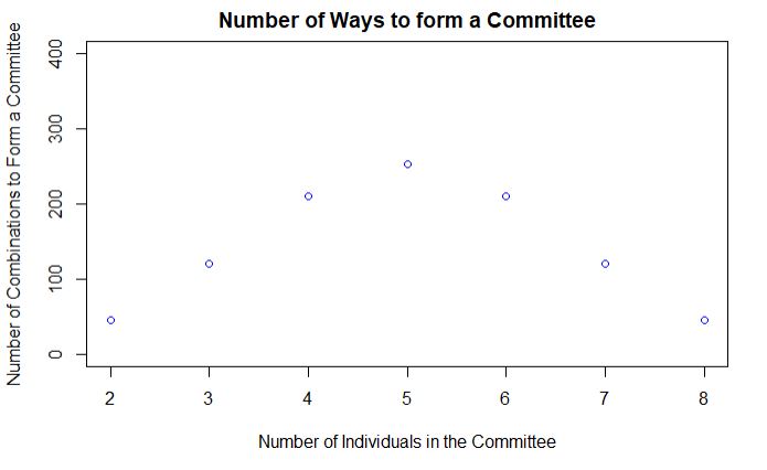
For 3-member teams, it comes out to be 10C3 or 120. The choice increases to the maximum for 5 (252 combinations), and then decreases symmetrically such that nCk = nCn-k (number of 3-member groups = number of 7-member groups and so on).

The following R code uses the function choose(n,k) to evaluate the binomial coefficient and plots the outcome.

committe <- function(n,k){
  choose(n,k)  
}

diff <- seq(2,8)
diff_com <- mapply(committe, diff, n = 10)

plot(x = diff, y = diff_com, main = paste("Number of Ways to form a Committee"), xlab = "Number of Individuals in the Committee", ylab = "Number of Combinations to Form a Committee", col = "blue", ylim = c(0,400))
It requires number crunching, and mental constructs don’t always help. In a study, when people were asked to make guesses, the median estimate of the number of 2-member committees was around 70; 8-member committees were at 20. So, imagining a few two-member teams were possible in mind, whereas 8-member groups were beyond its capacity.

Tversky, A.; Kahneman, D., Science, 1974 (185), Issue 4157, 1124-1131

T&K Stories – 3. Biases of Imaginability Read More »
T&K Stories – 2. Birth of Baby Boys

A certain town is served by two hospitals. In the larger hospital about 45 babies are born each day, and in the smaller hospital about 15 babies are born each day. As you know, about 50 percent of all babies are boys. However, the exact percentage varies from day to day. Sometimes it may be higher than 50 percent, sometimes lower.

For a period of 1 year, each hospital recorded the days on which more than 60 percent of the babies born were boys. Which hospital do you think recorded more such days?

b The larger hospital
b The smaller hospital
b About the same

Judgment under Uncertainty: Heuristics and Biases, Tversky and Kahneman

If you recall the law of large numbers, you would have guessed the correct answer, i. e. the smaller hospital. Because as the number of births increases, the gender of the baby comes closer to the expected percentage of 50.

If you still doubt, let’s run a simple Monte Carlo run using the following R code,

days  <- 365
birth <- 15
boy   <- 0.5
boys  <- replicate(days, {
  prob_birth <- sample(c(0,1), birth, prob = c((1-boy), boy), replace = TRUE)
  mean(prob_birth)*100
})

sum(boys > 60)

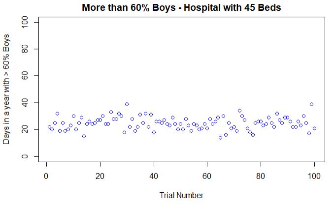
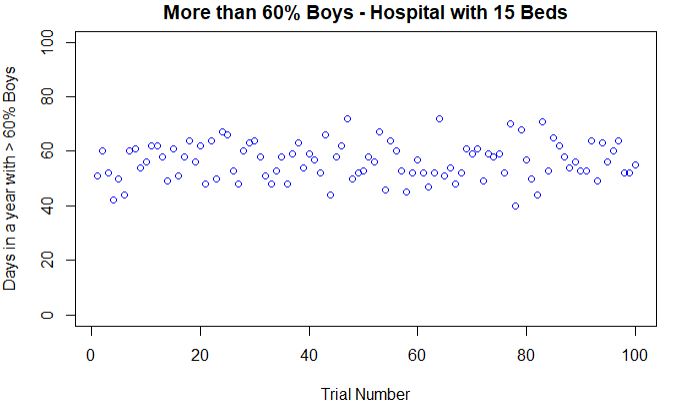
Run this code 100 times and plot the answers, the probabilities of a day in which more than 60% were boys:

Now, change the number of births to 45 and re-run the calculations:

What about more than 60% of girls?

Let me end this piece with this one. Which hospital do you expect more number of days with less than 40% of boys? No marks for guessing: it is still the small hospital.

Tversky, A.; Kahneman, D., Science, 1974 (185), Issue 4157, 1124-1131

T&K Stories – 2. Birth of Baby Boys Read More »

T&K Stories – 1. Librarian vs Farmer

“Steve is very shy and withdrawn, invariably helpful, but with little interest in people, or in the world of reality. A meek and tidy soul, he has a need for order and structure, and a passion for detail.”

Judgment under Uncertainty: Heuristics and Biases, Tversky and Kahneman

Following the clues above, your task is to guess if Steve is a farmer or a librarian.

A significant proportion of people may have guessed Steve was a librarian. Some of the others who chose farmer may have done it so out of suspicion of the build-up. 

Back to Bayes’ics 

Remember the Bayes’ theorem? If not, read my earlier post, The Equation of life.  

P(Lib|D) = P(D|Lib) x P(Lib) / [P(D|Lib) x P(Lib) + P(D|noLib) x P(noLib)]

Let us check the chance for the frequent answer – that Steve was a librarian – to be true (P(Lib|D)). I am ready to support the argument that all librarians fit this stereotype (P(D|Lib) = 1) if that was a concern. It is unlikely to be valid, but I give you that benefit of the doubt. Estimating the prior probability of librarian in a set of farmers and librarians (P(Lib)) is the task that needs data. Based on the available data in the public domain, in the US, that ratio is 0.026!

P(D|noLib) or the description fitting farmers is tricky, but I make an assumption least 10% of the farmer community can have shy and withdrawn men! P(noLib) is nothing but 1 – P(Lib). Substitute all the numbers

(1 * 0.026)/[(1 * 0.026)+(0.1 * 0.974)] = 0.21.

Even if all the librarians fit your mental stereotype, you are right only 20% of the time. To paraphrase what late Hans Rosling used to say: a chimp would do a better job; she picks the correct answer 50% of the time.

It’s not about Maths

The message here is not about the math, nor about the research required to get an accurate answer. It is only about being mindful about our biases and how much they can lead to inaccurate perceptions about others.

References

Tversky, A.; Kahneman, D., Science, 1974 (185), Issue 4157, 1124-1131

Librarians in the US

Professional Workforce in the US

Statistics farmers in the US

T&K Stories – 1. Librarian vs Farmer Read More »

Tversky and Kahneman – and the Paper that Challenged Our Judgements

Let me talk about an article that I want you to read. It is titled ‘Judgment under Uncertainty: Heuristics and Biases‘, published in Science 1974. The paper is about heuristics, the mental shortcuts to arrive at decisions, and its inherent problems in real life. And the consequence? Implicit biases to gambling-addiction, stereotyping to micro-inequities.

We have seen in the past few posts how unreliable our intuitions about conditional probabilities can be. The authors give many stories to expose the errors in judgements that we are carrying.

I will go through their stories one by one in the coming days, but first, you read the paper.

Tversky, A.; Kahneman, D., Science, 1974 (185), Issue 4157, 1124-1131

Tversky and Kahneman – and the Paper that Challenged Our Judgements Read More »

The risk from the New Variant

As calamities from another variant of Covid19 is looming large, the omicron, be prepared for more confusing news in the coming days. It is also the right time to introduce the word risk. Risk has a specific technical meaning. It is the product of the likelihood of something to happen and the consequence.

Risk = likelihood x consequence.

Compare the delta variant with ones that came earlier. From the data, anecdotal evidence by individuals and evolutionary arguments, it became the public narrative that the consequence of infection with delta was similar to, or even mildly less dangerous. Did it mean the same for the risk? We can’t say until we know the likelihood. Delta turned out to be more than double as contagious as earlier ones. So the overall risk was much more than the first.

The second common argument was the case fatality rate. The CFR, as it is commonly known, was not high, they argued, but forgetting that almost a third of humanity was going to get it. A small fraction of a large number is still sizeable.

Black Swan Event

An extreme example of risk is the black swan event – a concept introduced by Nassim Nicholas Taleb through his book that carried the same name. These are unpredictable events and has infinite consequences.

Was the Covid pandemic a black swan event? As per the author himself, it was not a black swan event. People had predicted viruses attacks like these, and there were, however hypothetical, opportunities to control the disease at its onset, had there been a few steps taken by the originating country – be it intervention at the start or by just being more transparent.

But September 11 was one of them. It was never anticipated, and the consequence was enormous and far-reaching.

Delta variant

Black Swan Theory

Covid19 and Black Swan

The risk from the New Variant Read More »

More On Prosecutors fallacy

Imagine a crime scene where the investigators were able to collect bloodstain. The sample was old, the DNA degraded, and the analysts estimated a relative frequency of 1 in 1000 in the population. Police found a suspect and got a DNA match. What is the chance that the suspect is guilty?

The prosecutor argues that since the relative frequency of the DNA match is 1 in 1000, the chance for the person to be innocent is 1 in 1000 and deserves maximum punishment. Well, the prosecutor made a wrong argument here. Imagine the city has 100,000 people in it. The test results suggest that there are about 100 people whose DNA can match the sample. So, the suspect is one of 100, and the chance of innocence only based on the DNA test is 99%.

Not Convinced? Let us use Bayes’ theorem.

P(INN|DNA) = P(DNA|INN)*P(INN)/ [P(DNA|INN)P(INN) + P(DNA|CRI)*P(CRI)]

P(INN|DNA) – the chance that the suspect is innocent given the DNA matches
P(DNA|INN) – chance of DNA match if the suspect is innocent = 1/1000
P(CRI) – prior probability that the suspect did the crime = 1 /100,000 (like any other citizen)
P(INN) – prior probability that the suspect is innocent = (1 – 1 /100,000)
P(DNA|CRI) – chance of DNA match given the suspect did the crime = 1 (100%)

P(INN|DNA) = (1/1000)* (1 – 1 /100,000) / ((1/1000)* (1 – 1 /100,000) + 1*(1/100000)) = 0.99

Does this mean that the suspect is innocent? Not either. The results only mean that the investigators must collect more evidence to file charges against the suspect.

More On Prosecutors fallacy Read More »

Prosecutors fallacy

We have seen that Bayes’ theorem is a fundamental tool to validate our beliefs about an event after seeing a piece of evidence. Importantly, it utilises existing statistics or prior knowledge to get to a conclusion. In other words, our hypothesis gets better representativeness by using Bayes’ theorem.

Take some examples. What are the chances that I have a specific disease, given that the test is positive? How good are my perceptions of a person’s job or abilities just by observing a set of personality traits? What are the chances that the accused is guilty, given that a piece of evidence is against her?

Validating hypotheses based on the available evidence is fundamental to investigations but is way harder than they appear, partly because of the illusion of the mind that confuses the required conditional probability with the opposite. In other words, what we wanted to find is a validation of the hypothesis given the evidence, but what we see around us is the chance of evidence if the hypothesis is true, because often, the latter is part of common knowledge.

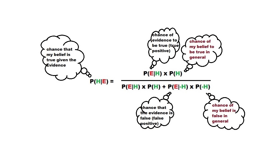
To remind you of the mathematical form of Bayes’ theorem

Note that the denominator on the right-hand side is the probability of the evidence P(E)

Confusion between P(H|E) and P(E|H)

What about this? It is common knowledge that a running nose happens if you have a cold. Once that pattern is wired to our mind, the next time when you get a running nose, you assume that you got a cold. If the common cold is rare in your location, as per Bayes’ theorem, the assumption that you made require some serious validation.

Life is OK as long as our fallacies stop at such innocuous examples. But what if that happens from a judge, hearing the murder case? It is the classic prosecutor’s fallacy in which the size of the uncertainty of a test against the suspect is mistaken as the probability of that person’s innocence.

chances of crime, given the evidence = chance of evidence, given crime x (chance of crime/chance of evidence). Think about it, we will go through the details in another post. 

Prosecutors fallacy Read More »

The Big Short and The Assumption of Independence

In the last post, we have seen how banks make money by lending. To get estimates of profits and probabilities, we have assumed two conditions – independence and randomness. This time we look at cases where both these assumptions don’t hold.

Our bank is now making about 1.8 million annual returns with 2000 customers, who have been handpicked for their high credit scores and predictability to repay.

Want for More

An idea was proposed to the management to expand the firm and to increase the customer base. The argument was that even though adding more customers can reduce the predictability of defaulting, the risks could be managed by raising the interest rate a bit higher. Assurance was given that even for an assumed default rate of 5%, which is double the existing, by increasing the interest rate to 6.3%, the bank can make up about 8 million with 99% confidence. She has rationalised her calculations based on the law of large numbers, that the bank is unlikely to miss the target.

The expected value of profit = [interest rate x profit per loan x (1-default rate) – cost per foreclosure x default rate] x total number of loans.

For 20,000 loans, this will mean

[0.063 x 9000 x (1-0.05) – 100,000 x (0.05)] x 20,000

an earning of about 8 millions!

She further shows a plot of the simulation to support her arguments.

It convinced the management, and the company is now on an aggressive lending campaign. The firm has now 20,000 customers and makes a lot of money. A few months later comes a global financial crisis, and the firm is now bankrupt.

Assumption of Independence

To understand what happened to the bank, we should challenge the assumptions used in the original statistical calculations, especially the independence of variables – that one person defaults does not depend on the other. When there are many borrowers with varying capacities to repay, such crises prove detrimental to the business.

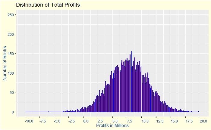
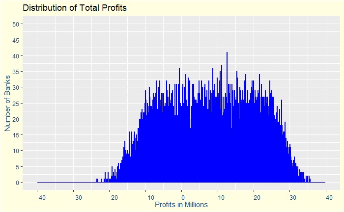
Assume a 50:50 chance, up or down, for everyone to default by a tiny fraction + / – 0.01 (1%) or between 0.04 and 0.06. Note that the average risk of default is still 5% but are no longer independent. Subsequently, the overall chances for making a loss has moved from 1% to 31%, but the average return is still around 8 million. A plot of the distribution of profits is below.

The plot is far from a uniform distribution as the central limit theorem would have predicted using an assumption of complete independence of variables.

The Big Short and The Assumption of Independence Read More »

Interest Rates and How not to Lose Money

In the previous post, we have seen how banks can lose money when they do the business of making money by disbursing loans. This time we will see how banks manage that risk by setting an interest rate for every loan they give. It means every lender needs to pay a fixed proportion of the borrowed money to the bank as a fee.

How does a bank set an internet rate? It is a balance between two opposing forces. If the rate is too low, it will not adequately cover the risk of defaults, and if it is too high, it could keep the customers away from taking loans.

Take the case of 10,000 banks each lends 90,000 dollars per customer to 2000 customers. Let’s say the bank sets an interest rate of 3% on the loans. After running Monte Carlo simulations, we can see the following.
The bank can earn a net profit of about 0.26 mln, but there is a 35% that it will lose money. In other words, 3500 banks won’t make money. The plot below describes this scenario.

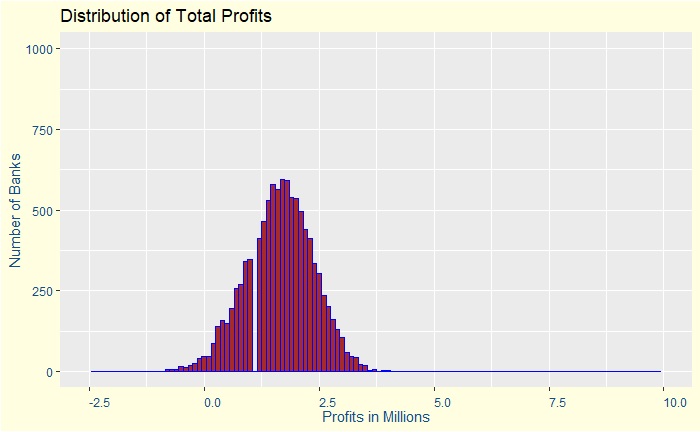
Increase the interest rate to 3.8%. The expected profit is 1.6 mln, and there is about 1% of losing money. That sounds reasonable for a person to run the business. See below for the distribution.


Increase the interest rate to 5% and the profit if we manage to have all the customers intact is 3.77 mln and almost 0% chance of losing money. But a higher interest rate can drive customers away from this bank. Suppose three fourth of the customers have gone to other banks. The profit from 500 customers is less than a million and also there about 0.8% of losing money. Note that fluctuations increase to our estimations – net profits and the chances of making money – as the numbers are smaller (the opposite of the law of large numbers).

Interest Rates and How not to Lose Money Read More »

The Central Limit Theorem

The Central Limit Theorem (CLT). It has intrigued me for a long time. The theorem concerns independent random variables, but it is not about the distribution of random variables. We know that a plot of independent random variables will be everywhere and should not possess any specific pattern. The central limit theorem is about the distribution of their sums. Remember this.

Let us take banks and defaulters to prove this point. Suppose a bank gives away 2000 loans. The bank knows that about 2.5% of the borrowers could default but does not know who those 50 individuals are! That means the defaulters are random. They are also independent. These are two highly debatable notions; once in a blue moon, these assumptions will prove to be the bank’s end. But we’ll deal with it later.

So, what is the distribution of losses to this bank due to defaults? Before that, why is it a distribution and not a fixed number, say, 50 times the loss per foreclosure? Or if the loss per foreclosure is 100,000 per loan, the total loss is 50 x 100,000 = 5 million. A fixed number. That is because a 2.5% default rate is a probability of defaulting, not a certainty. If it is a probability, the total loss to the bank is not a fixed amount but a set of random numbers.

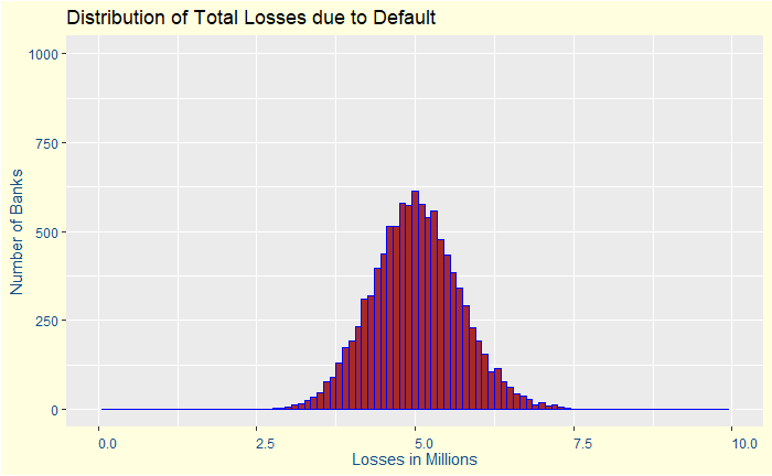
Let’s disburse 2000 loans to people and collect data from 10,000 banks worldwide! How do we do it? By Monte Carlo simulations. The outcome is given below as a plot.

This is the Central Limit Theorem! To put it in words, if we take a large number of samples from a population, and these samples are taken independently from each other, then the distribution of the sample sums (or the sample averages) follows a normal distribution.

The Central Limit Theorem Read More »