So far, we have been accepting the notion that the posterior probability from the Bayes’ equation becomes the prior when you repeat a test or collect more data. Today, we verify that argument. What is the chance of having the disease if two independent tests turned positive? Let’s write down the equation.
Since the two tests are independent, and the marginal probability of the two positive tests is similar, we can write P(++|D) as the joint probability, P(+|D)*P(+|D). The same is true for the false positives, P(++|nD). Substituting all of them, we get
P(+|D) is your sensitivity, P(+|nD) is 1 – specificity and P(D) is the assumed prior.
Now, we will go to the original proposition of the posterior becoming the next prior. The probability of having the disease given the second test is also positive is given by
Yes, posterior is the new prior! If you generalise the equation for n number of independent tests,
I guess you remember the story of Sophie that we encountered at the start of our journey with the equation of life. She has tested positive during a cancer screening but found that the probability of the illness was about 12% after applying Bayes’ principles. There was nothing faulty about the test method, which was pretty accurate, at 95% sensitivity and 90% specificity. Now, how many independent tests does she need to undertake to confirm her illness at 90% probability?
Assume that her second test was positive: The probability for Sophie to have cancer, given that the second test is also positive,
The updated probability has become 56% (note we have used 12.6%, which is the posterior of the first examination, as the prior and not the original 1.5%). Applying the equation one more time for a positive (third by now) test, you get
So the answer is three tests to get a high level of confidence.
You may recall that the prior probability used in the beginning was 1.5%, based on what she found in the American Cancer Society publications. What would have happened if she did not have that information? She still needs a prior. Let’s use 0.1% instead. Let’s work on the math, and you will find that about 89% probability can reach in the fourth test, provided all are positive. Therefore, an accurate prior is not that crucial as long as you follow up with more data collection, which is the power of the Bayesian approach.
We have seen the Monty Hall problem in an earlier post. This time, instead of 3, we have four doors. There is $1000 behind one door, -$1000 behind another (you lose $1000), and two other doors have nothing ($0). Like in the previous game, you choose one door, and then the game host opens a door that contains nothing. You have an option to change to one of the other closed doors now. What will you do?
No Change
In the beginning, before hosts reveals the $0 door, the probabilities are P($1000) = 1/4, P($0) = 1/2 and P(-$1000) = 1/4. The expected return is (1/4) x $1000 + (1/2) x $0 + (1/4) x -$1000 = $0. After the clue, if you still don’t want to change, this remains the case.
Change
Here, we use solution 2, the argument method, of the Monty Hall problem. Before you get the clue, the chance that you chose the $1000 door is 1/4, and that the prize was outside your choice is 1 – 1/4 = 3/4. After the clue, that probability of 3/4 sits behind two doors. In other words, if you shift, the chance of getting $1000 is 3/8. Using similar arguments, we shall see that the chance of losing became 3/8, and for $0 is 1/4. The expected return is (3/84) x $1000 + (1/2) x $0 + (3/8) x -$1000 = $0.
Will you change?
Well, it depends on your risk appetite. The chance of winning and the chance of losing have increased. But the expected returns remained the same, at zero. Or the risk has increased if you shift. If you are risk-averse, stay where you are!
Decision-making in groups often suffers from what is known as the Arrow’s impossibility problem. Named after the American Economist Kenneth Arrow, this theory says that if a decision is made by a group of individuals who are not run by a dictator, through sincere voting, they may reach a state of non-transitive preference even if they are all rational.
The statement sounds very complicated. Let’s look at each of those words. First, something about the group – they are free and have clear preferences. The second one is non-transitive preference. To understand this, we must understand what transitive preferences are.
Transitive preference
Rational decision-makers have transitive preferences. That means if a decision-maker prefers A over B, then B over C, it must be that she prefers A over C. A sort of mathematical consistency. But this is so if the decision-maker is one person. What can happen if there is more than one? Take this example of three members of a local committee, Mrs Anna, Mr Brown and Miss Carol. The following represent their choices on what they prefer to build for the local community this year.
Anna
Brown
Carol
First Preference
School
Library
Playground
Second Preference
Library
Playground
School
Third Preference
Playground
School
Library
The committee votes for pair-wise comparison. The first is school vs library. Anna and Brown vote for their first choices, the school and the library, respectively, and Carol for school (because the library is her least preferred ). The school won 2-1.
The school vs playground happens next. The votes go through a similar process, and the playground wins this time, thanks to Mr Brown; the school was his least preferred option.
You may conclude that the committee should build a playground because it beat the school that defeated the library. But before that, they have to do the final voting- the library vs the playground. Since it was sincere voting, as you expected, the library won by 2 to 1 as Anna, the decider, broke the tie. And we ended up in a non-transitive situation.
Most of us acknowledge the need to be objective; in what we believe or what we decide. Yet, we find it tough to follow the path of true objectivity as the pull from the value system is so strong. And we settle for results that fit with our current ideas.
My-side objectivity
And that is confirmation bias. It is a state in which individuals will search, accept and interpret information that favours their existing beliefs. Traditionally it required active selection from the individual, be in the newspaper she chooses, the books she reads etc.
Filter bubble
Naturally, the bias also requires us to ignore the evidence that does not fit our liking. And that used to be a difficult job. But that is past. With the introduction of filter bubbles or those algorithms that choose the feed for you, confirmation has reached a different level. The algorithm practically takes the decision, on your behalf, on what to click on and what not to.
Recency bias is another common type of cognitive bias in which people’s decisions are influenced by what happened in recent times. An example is the bull and bear runs of the stock market. When the market is having a good time, people assume that it will continue and increase their investments, attracting even more into the bubble. On the other hand, when the market crashes, the trend reverses as more people want to sell, expecting the doom to continue. A lot of analysts, unaware of the bias, carry this fallacy and use the term momentum, a term borrowed from physics, to describe this phenomenon.
Another example is the mass cancellations after aircraft crashes. A recent news report says the cancellation, of close to 9000 flights, following the incident of a China Eastern Airlines flight in March this year. Interestingly this was the first fatal airliner incident in China in the last 12 years!
Availability bias is a mental shortcut for decision making that uses what comes to mind based on your impression, i.e. examples that are easily available to you to visualise. The following puzzle from Tversky and Kahneman is a nice one to illustrate this.
Look at the above two pictures and draw structures starting from the top row to the bottom by passing through one and only one X in a row. If you are not entirely sure about the task, let me illustrate it with examples. The following picture gives one such construction on each.
What comes to mind
If your answer is figure 1, then you are not alone. 46 out of 56 participants thought figure 1 has more paths than figure 2. Their median estimate was 40 in Fig 1 and 18 in Fig 2.
A permutation problem
It is a permutation problem that doesn’t need any guessing. Fig 1 calls for 8 ways to draw connections, 3 at a time or a total of 8 x 8 x 8 = 83 = 512 possibilities. The second one? Well, 2 ways, 9 at a time, 29 = 512 (2 x 2 x 2 x 2 x 2 x 2 x 2 x 2 x 2)!
Convincing the bank if you don’t have money or collateral is difficult, if not impossible. It is now easier for the bank to reach its subgame-perfect Nash equilibrium by rejecting the application. Here the bank has done nothing wrong as its primary goal was to protect its business. But in the process, it made the poor out of the credit market, eventually throwing them into a downward spiral. On the other hand, the bank was far more confident with the rich because of the collateral.
Bangladeshi economist Muhammad Yunis, who later got the Nobel Peace Prize for this work, broke this spiral by founding a community development bank, Grameen Bank, employing the microcredit system.
16 Decisions
The banking system works by giving several small loans to a pool of interconnected people. Then, instead of creating any legal framework, the Grameen bank laid a value system by sixteen decisions. Those are aimed to foster discipline, community building, saving, and sustainability.
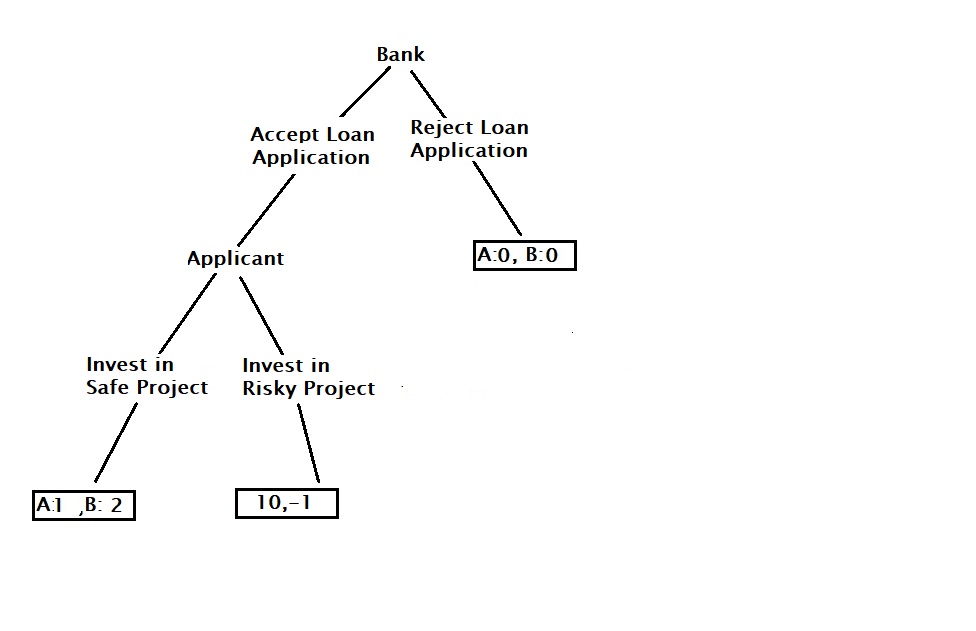
The interaction between a lender and a borrower is an example of a sequential-move game. The game tree, along with the payoffs, is shown below. A represents the applicant, and B represents the bank.
It is a sequential move game because the applicant gets the chance to invest in the project of her choice only after the bank has released the money.
Based on the payoff, it is easy to find that the bank gets a good deal only when the applicant invests in a safe project. If the bank doubts the applicant’s intention, it will reject the application straight away. In such a case, the applicant has only two choices: 1) convince the bank that she would invest in a safe project, 2) give collateral to guarantee the bank.
We have seen how coordination failure has led the game to a simultaneous move. Now, think about another scenario where there was no network failure, and the communication was possible between A and B. This can lead to another type of game; the sequential move. But before we move on to that, let us look at the original payoff matrix.
B
Football
Dance
A
Football
A:10, B:5
A:0, B:0
Dance
A:0, B:0
A:5, B:10
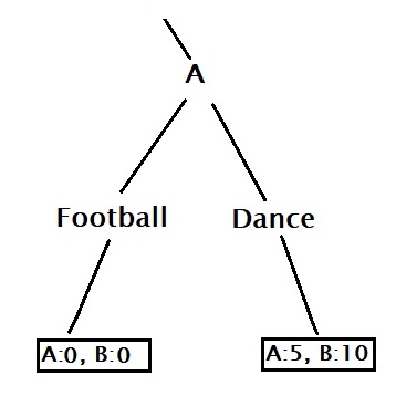
In this case, B finishes her job earlier, reaches the dance venue and calls up A. So B becomes the first mover, and A’s strategy now depends on the following game tree (full version).
Now that B has made her move, i.e. dance, the subgame has only the A’s part of the tree.
And the loving A has only one option to select and maximise the couple’s happiness! It has become a subgame perfect Nash equilibrium, favouring the early mover, B in this case.
Not a guaranteed success
Although the present story tells otherwise, there are no rules to guarantee maximum payoff for the first mover. There are several examples where followers benefitted from early movers’ mistakes, especially in businesses that require heavy R&D and are high in fast-evolving technology content. As per this HBR article, gradually evolving technologies and market gives the early mover better chances.


![\\ P(D|2nd +) = \frac{P(2nd +|D)*P(D|1st+)}{P(2nd +|D)*P(D|1st+) + P(2nd+|nD)*(1-P(D|1st+))} \\ \\ \text{where, } \\ \\ P(D|1st+) = \frac{P(+|D)*P(D)}{P(+|D)*P(D) + P(+|nD)*(1-P(D))} \\ \\ \text{since these tests are independent}, P(2nd +|D) = P(+|D) \text{. Substituting, } \\ \\ P(D|2nd +) = \frac{P(+|D)*P(D|1st+)}{P(+|D)*P(D|1st+) + P(+|nD)*(1-P(D|1st+))} \\ \\ = \frac{P(+|D)* [ \frac{P(+|D)*P(D)}{P(+|D)*P(D) + P(+|nD)*(1-P(D))} ] }{P(+|D)* [ \frac{P(+|D)*P(D)}{P(+|D)*P(D) + P(+|nD)*(1-P(D))} ] ) + P(+|nD)*(1- [ \frac{P(+|D)*P(D)}{P(+|D)*P(D) + P(+|nD)*(1-P(D))} ] )} \\ \\ \text{expanding and cancelling similar terms,} \\ \\ P(D|2nd +) = \frac{P(+|D)*P(+|D)*P(D)} {P(+|D)*P(+|D)*P(D) + P(+|nD)*(1-P(D))} = P(D|++)](https://thoughtfulexaminations.com/wp-content/ql-cache/quicklatex.com-a9ed4c7fc65cf1f46e1a6a9b58fb4d10_l3.png "Rendered by QuickLaTeX.com")