Decision Making

Shark Attack

This post will run in three parts. Here, we take a Bayesian inference challenge and analyse it analytically and numerically. I have followed the book “Bayesian Statistics for Beginners” by Donovan and Mickey for reference.

Bayesian Inference

The objective of Bayesian inference is to update the probability of a hypothesis by incorporating new data. The generic form of the Bayes’ theorem is written as:

P(\theta|Data) = \frac{P(Data|\theta) P(\theta)}{\int P(Data|\theta) P(\theta) d\theta}

The left-hand side of the equation represents the posterior distribution of a single parameter, theta, given the observed data. The first term on the numerator is called the likelihood, and the second term is the prior distribution (the existing knowledge before the arrival of the new data) of the parameter. We will soon see what I meant by parameter and how the (distribution) functions for the likelihood and prior are selected. Remember, the integral in the denominator is a constant; we will use that information soon.

Sharks and Poisson

Now the problem you want to solve: it is known that, on an average year, five shark attacks happen in a particular place. Last year it rose to ten. Do you think it is abnormal, and how do you update your database based on this data?

Shak attacks are rare. And they follow no pattern; in other words, one episode is independent of the previous one. Yes, you are guessing it right; I want to use the Poisson distribution to describe the likelihood of shark attacks. Although the word “poisson” means fish in French, the distribution got its name after the famous French mathematician Simeon Poisson!

The Parameter

In our case, based on the historical data, five attacks occur a year. Now, can the average five justify seeing ten last year? You either use the formula as seen in an earlier post or the R code, dpoise(10, 5). The answer is ca. 0.018. What about using a parameter value of 6 or 8? If you plug in those numbers, you will find they also lead to non zero probabilities. In other words, it is better to use a set of numbers (also called a distribution) instead of a single number as your prior. A gamma distribution can provide that set for two reasons, 1) it can give a continuous range of parameter values you wanted 2) the function is well suited with Poisson for solving the integral of the Bayes’ equation analytically. If you want to know what I meant, check this out.

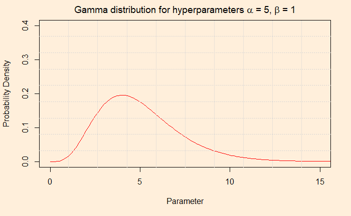
The Gamma distribution function has two hyperparameters, alpha and beta. We use the word hyperparameters to distinguish from the other (theta), which is the unknown parameter of interest. Alpha/beta gives the mean. In our case, we settle for alpha = 5 and beta = 1 for the prior. The average (5/1 = 5) is matching with the existing data. You may as well consider 10 and 2, which also gives a mean of 5, but we stick to 5 and 1. Before we go and do the analysis, which is in the next post, check the parameter values that we will input to the Poisson to use.

Yearly Worldwide Shark Attack Summary

Shark Attack Read More »

Biases As Part of our Survival

People unaware of their own biases pose a clear threat to quality decision making. And we have discussed biases several times in the past. However, biases are also a result of our need to minimise energy spent on the thinking process. We will see what this means.

Scientists have hypothesised an explanation for this phenomenon along the lines of cognitive operations of the human system. They classify two types of thinking processes. They are 1) System one or intuitive thinking and 2) System two or reflective thinking.

In the first case, our actions flow effortlessly. Such as eating a piece of cake! Since we have evolved this way, it is not a complete surprise that energy-saving conserving modes of thinking got the default status (the brain consumes 20% of the body’s energy).

Reflective thinking, on the other hand, requires more energy. These are deliberate and slow, and you do it when the stakes are high. The primary focus is to reduce error, and therefore you are willing to spend your valuable energy. Remember our past as hungry hunter-gatherers.

To give an example, when someone learns how to ride a bike, “a very risky affair”, she is in system-two mode. A year later, as a master biker now, riding is her second nature, and it is now a system one process.

Biases As Part of our Survival Read More »

Whose Fault was It?

A company gets their tools from three factories, 10% from F1, 50% from F2 and 40% from F3. The fault rates of the three factories are 2.5%, 1.5% and 1%, respectively. If the company finds one of the tools defective, from which factory is it likely?

Let’s write down things in the proper format and test the probabilities, one by one. Let P(F1|D) be the probability that the tool came from F1 given the information (that it is faulty), P(D|F1), the fault rate of F1 and P(F1) is the prior chance of F1 in the company.

\\ P(F1|D) = \frac{P(D|F1)*P(F1)}{P(D|F1)*P(F1) + P(D|F2)*P(F2) + P(D|F3)*P(F3)}  \\ \\ P(F2|D) = \frac{P(D|F2)*P(F2)}{P(D|F1)*P(F1) + P(D|F2)*P(F2) + P(D|F3)*P(F3)}  \\ \\ P(F3|D) = \frac{P(D|F3)*P(F3)}{P(D|F1)*P(F1) + P(D|F2)*P(F2) + P(D|F3)*P(F3)}

I guess you already know that I applied Bayes’ theorem to each factory. Now, add numbers and solve.

\\ P(F1|D) = \frac{0.025*0.1}{0.025*0.1 + 0.015*0.5 + 0.01*0.4}  = \frac{0.0025}{0.014} = 0.18\\ \\ P(F2|D) = \frac{0.015*0.5}{0.025*0.1 + 0.015*0.5 + 0.01*0.4}  = \frac{0.0075}{0.014} = 0.54\\ \\ P(F3|D) = \frac{0.01*0.4}{0.025*0.1 + 0.015*0.5 + 0.01*0.4}  = \frac{0.004}{0.014} = 0.29

The tool is more likely to have come from F2.

Whose Fault was It? Read More »

Two Envelope Problem

Consider this: there are two envelopes on the table containing some cash. You don’t know how much it is, but you know that one contains twice the amount as the other. You were given one of them at random. You have two choices: open the one you got and take the cash, or switch to the other. What will you do?

Expected Value

Naturally, you will go for the expected value of a switch, and if that is greater than the money at hand, you will make the exchange. Let the amount of money inside your envelope be X. You doubt the other envelope has 2X or X/2 amount. And they are equally likely (probability of half). The Expected value, in that case, is (1/2)x2X + (1/2)x(X/2) = X + (1/4)X > X. So, you switch, right?

The problem with the problem

No, you will not. Think about the issue with a swap. After making the switch, you can make the same expected value calculations for the original envelope, draw the same conclusion, and switch back—and you do it forever!

The problem, in reality, involves two conditional probabilities and needs to be solved separately. First, you assume that the second envelope contains less than the first. In the second case, you consider the opposite, i.e., the second envelope holds more than the first. You multiply the respective probabilities to get the answer.

E(2nd) = V(2nd | 1st < 2nd)xP(1st < 2nd) + V(2nd | 1st > 2nd) x P(1st > 2nd).
For X and 2X, E(2nd) = 2X(1/2) + X(1/2) = 1.5X.

Naturally, if X and 2X are the two options, the average value with the first envelope is not X, but (X+2X)/2 = 1.5X

They match, and no need to switch!

Two Envelope Problem Read More »

Waiting for Heads

The last time, we saw the expected waiting times of sequences from coin-flipping games. Today, we will make the necessary formulation to theorise those observations.

We have already seen how the expected values are calculated. In statistics, the expected values are the average values estimated by summing values multiplied by the theoretical probability of occurrence. Start with the simplest one in the coin game.

Consider a coin with probability p for heads and q (= 1-p) for tails. Note that, for a fair coin, p becomes (1/2).

Expected waiting time for H

You toss a coin once: it can land on H with probability p and T with q or (1 -p). If it is H, the game ends after one flip. The value (for the time to wait) becomes 1, and the expected value, E(H), for an H start is p x 1. On the other hand, if the flip ends up with T, you start again for another flip. In other words, you did 1 flip, but back to E(H). The expected value, in this case, is (1-p)x(1 + E(H)). The final E(H) is the sum of each starting possibility.

\\ E(H) = p*E(H1) + q*E(T1)\\ \\ E(H) = p*1 + (1-p)*(1 + E(H)) \\ \\ p*E(H) = p + 1 - p \\ \\ E(H) = \frac{1}{p} = 2 \text{, for a fair coin (p = 1/2)}

This should not come as a surprise. Since p is the probability of getting heads (say, 1/2), you get an H on an average 1/p (2) flip if you flip several times.

Expected waiting times for HT

We follow the same logic again. You made one flip (1), and you have two possibilities as starting – p x E(HT|H) and q x E(HT|T). HT|H means H followed by T given H has happened. For the second flip, you either start from the state of H or from the state of T.

\\ E(HT) = 1 + p*E(HT|H) + q*E(HT|T) \\ \\ \text{from the state of H, } \\ \\ E(HT|H) = p*(1 + E(HT|H)) + q*1 \\ \\ E(HT|H) = \frac{p + q}{1 -p} = \frac{1}{0.5} = 2\\ \\ \text{from the state of T, } \\ \\ E(HT|T) = p*(1 + E(HT|H)) + q*(1 + E(HT|T)) \\ \\ E(HT|T) = 0.5*(1 + 2) + 0.5*(1 + E(HT|T)) \\ \\ E(HT|T) = \frac{0.5*(1 + 2)}{0.5} + \frac{0.5}{0.5} = 4 \\ \\ E(HT) = 1 + p*2 + q*4 = 1+1+2 = 4

Expected waiting times for HH

We’ll use a different method here.

\\ \text{If the first toss is a T, } \\ \\ term1 = q*(1+E(HH)) \text{; start again with the same expected time, E(HH), after the first T}\\ \\ \text{First toss is an H and the two tosses are HT } \\ \\ term2 = p*q*(2+E(HH)) \text{; start again after the second, T}\\ \\ \text{First toss is an H and the two tosses are HH, and you win in 2 tosses} \\ \\ term3 = p*p*2 \\ \\  E(HH)) = term1 + term 2+ term3 = q*(1+E(HH)) + p*q*(2+E(HH)) + p*p*2  \\ \\ E(HH)) = 0.5 + 0.5*E(HH)) + 2*0.5*0.5 + 0.5*0.5*E(HH) + 0.5*0.5*2 \\ \\ E(HH)) = \frac{0.5+2*0.5*0.5+0.5*0.5}{0.25} = \frac{0.5+2*0.5*0.5+0.5*0.5*2}{0.25} = \frac{1.5}{0.25} = 6

Waiting for Heads Read More »

Coin Flip Game

We are back to our favourite topic – coin-flipping. Anna and Ben are playing a game of flipping coins. They aim for a pattern and whoever gets it there wins. Anna chooses head-tail (HT) and Ben for head-head (HH). Who do you think will win?

You may assume since the probability of getting HT or HH in two tosses is the same, i.e., 1 in 4, the chances of winning should be identical. But the game is not about two tosses. The game is about several tosses and then counting who got the most. Let’s do this game first before getting into any theories. The following R code executes the game 10000 times, each with 5000 flips at a time, and calculates the number of times they get their respective patterns.

library(stringr)

redo <- 10000
flip <- 5000

streak <- replicate(redo, {
toss <- sample(c("H", "T"), flip, replace = TRUE, prob = c(1/2,1/2))
toss1 <- paste(toss,collapse=" ")
count <- str_count(toss1, c("H H"))

})

mean(streak)


streak <- replicate(redo, {
toss <- sample(c("H", "T"), flip, replace = TRUE, prob = c(1/2,1/2))
toss1 <- paste(toss,collapse=" ")
count <- str_count(toss1, c("H T"))

})

mean(streak)

The answer I got was 833.17 for Ben (HH) and 1249.76 for Anna (HT). Divide the number of flips with these numbers, and you get the average waiting times for the pattern. They are 5000/833.17 = 6 and 5000/1249.76 = 4. So, on average, Anna needs to wait for four flips, and Ben needs six before getting the pattern.

Pattern of three

Let us extend this for 3-coin games. Using the following code, we find the average waiting time for the three patterns – HHT, HTH, and HHH.

```{r}
library(stringr)

redo <- 10000
flip <- 5000

streak <- replicate(redo, {
toss <- sample(c("H", "T"), flip, replace = TRUE, prob = c(1/2,1/2))
toss1 <- paste(toss,collapse=" ")
count <- str_count(toss1, c("H H T"))
})

flip/mean(streak)


streak <- replicate(redo, {
toss <- sample(c("H", "T"), flip, replace = TRUE, prob = c(1/2,1/2))
toss1 <- paste(toss,collapse=" ")
count <- str_count(toss1, c("H T H"))
})

flip/mean(streak)

streak <- replicate(redo, {
toss <- sample(c("H", "T"), flip, replace = TRUE, prob = c(1/2,1/2))
toss1 <- paste(toss,collapse=" ")
count <- str_count(toss1, c("H H H"))
})

flip/mean(streak)

The waiting times are 8, 10 and 14 flips, respectively, for HHT, HTH and HHH.

Chances not identical

We will look at the theoretical treatment in another post. But first, let us try and understand it qualitatively. While the probability of getting both those two-coin sequences (or three in the second game) may be the same, the game they played takes different pathways depending on each outcome.

Look at the game from Anna’s point of view (she needs HT to win): Imagine she starts with H. The next can be an H or a T. If it is a T, she wins. But if she gets an H, she doesn’t win, but a win is just a toss away, as there is a 50% chance for her to get a T in the next flip. In other words, her failure gives her a headstart for the next.

On the other hand, Ben also starts with an H. Another head, he wins, but a tail, he needs to start all over again. He must get an H and aim for another H. A 25% chance of that happening after a failure.

Coin Flip Game Read More »

Cars No Safer

Calculating the risk numbers for passenger cars is a lot harder than the air. First, the data gathering is more challenging, thanks to the sheer number of vehicles on the road. The next thing is to estimate the number of car crashes a year. But, let’s make an attempt.

As per wiki, globally, about 1.4 billion motor vehicles are in use; a billion of them are cars. We don’t know how many journeys those make. Assuming an average of 100 days, you get 200 billion trips a year.

We use some shortcuts to estimate the number of crashes involving cars. India, which accounts for 11% of global death from road accidents, reports 150,000 fatalities from 450,000 incidents in a year. By extending the logic to the global scale, for the 1.3 million deaths every year, we estimate the incidents to be four million. We try yet another way of estimation. About 50 million injuries happen every year from vehicles and let’s assume half of them involve people travelling in the car (same ratio of reported death). The rest of them involves pedestrians and cyclists. Assuming an average of 3 people inside, we can estimate 25/3 = 8.3 million cars involved in incidents.

In the same way, 1.3 million deaths every year translates to 650,000 involving car travellers. That suggests a maximum of 650,000 fatal incidents and a minimum of 200,000 fatal incidents. Assume a mid-value of 400,000. Let’s compile all these (reported and assumed) into a table.

ItemData
# of car trips200 bln
(estimated)
# road incidents4 – 8 mln
(estimated)
# fatal incidents400,000
(estimated)
# deaths650,000
(estimated)
# passengers 600 bln
(estimated)
average trip length20 km
(estimated)
passenger-km12000 bln-km
(estimated)

Calculated quantities

MetricData
Incidents per trip20 – 40
(per million trips)
Fatal incidents per trip2
(per million trips)
Fatality per trip3.2
(per million trips)
Fatality per passenger-km54
(per billion-km)
Fatality per passenger0.81
(per million passengers)

Now compare these with what we had estimated previously for the air.

Comparison – air travel

MetricData
Incidents per trip3.13
(per million trips)
Fatal incidents per trip0.2
(per million trips)
Fatality per trip14.4
(per million trips)
Fatality per passenger-km0.06
(per billion-km)
Fatality per passenger0.13
(per million passengers)

Looks like air travel is safer on all counts.

References

[1] http://www.rvs.uni-bielefeld.de/publications/Reports/probability.html
[2] https://economictimes.indiatimes.com/news/politics-and-nation/india-tops-the-world-with-11-of-global-death-in-road-accidents-world-bank-report/articleshow/80906857.cms
[3] https://en.wikipedia.org/wiki/Aviation_accidents_and_incidents
[4] https://www.who.int/news-room/fact-sheets/detail/road-traffic-injuries
[5] https://www.icao.int/annual-report-2019/Pages/the-world-of-air-transport-in-2019.aspx
[6] https://data.worldbank.org/indicator/IS.AIR.PSGR
[7] https://en.wikipedia.org/wiki/Aviation_safety
[8] https://accidentstats.airbus.com/statistics/fatal-accidents
[9] https://injuryfacts.nsc.org/home-and-community/safety-topics/deaths-by-transportation-mode/
[10] https://www.sciencedaily.com/releases/2020/01/200124124510.htm

Cars No Safer Read More »

Riskier Flights

That flight travel is one of the safer modes of transportation is a foregone conclusion. Yet, there seems to be some confusion about the risk of taking flights versus, say, cars. Therefore the comparison requires a reevaluation.

The first question is: what is the right metric to use? Is it the number of fatalities per passenger boarding? Or is it the number of accidents/deaths per boarding? Yet another one is the number of accidents/deaths per passenger-kilometre travelled. Let’s make some (gu)estimates on each of these.

Available data

ItemData
# of flights40 mln (2019)
# aviation incidents125 (2019)
# fatal accidents8 (2019)
# aviation deaths575 (2019)
# passengers 4500 mln (2019)
average trip length2000 km
passenger-km9000 bln (2019)

Calculated quantities

MetricData
Incidents per trip3.13
(per million trips)
Fatal incidents per trip0.2
(per million trips)
Fatality per trip14.4
(per million trips)
Fatality per passenger-km0.06
(per billion-km)
Fatality per passenger0.13
(per million passengers)

Risk of air travel

In my option, the right metric is either the number of incidents per trip or the number of fatal incidents per trip. And probably the difference between road vs air. In air travel, the distance covered or the number of hours in the air are not the prime variable for incidents; riskier parts of a flight are the takeoff and landing, each of which happens once every trip, however brief or lengthy the travel be.

Comparison with the road

So how does it compare with road travel? That is a bit more complex as the data are hard to come by, requiring a lot of assumptions. Also, the risk of road travel has not distributed the way it is for the air. We’ll visit those in another post.

References

[1] http://www.rvs.uni-bielefeld.de/publications/Reports/probability.html
[2] https://economictimes.indiatimes.com/news/politics-and-nation/india-tops-the-world-with-11-of-global-death-in-road-accidents-world-bank-report/articleshow/80906857.cms
[3] https://en.wikipedia.org/wiki/Aviation_accidents_and_incidents
[4] https://www.who.int/news-room/fact-sheets/detail/road-traffic-injuries
[5] https://www.icao.int/annual-report-2019/Pages/the-world-of-air-transport-in-2019.aspx
[6] https://data.worldbank.org/indicator/IS.AIR.PSGR
[7] https://en.wikipedia.org/wiki/Aviation_safety
[8] https://accidentstats.airbus.com/statistics/fatal-accidents
[9] https://injuryfacts.nsc.org/home-and-community/safety-topics/deaths-by-transportation-mode/
[10] https://www.sciencedaily.com/releases/2020/01/200124124510.htm

Riskier Flights Read More »

A Laplace Equation Named Bayes

You may be wondering at the title of this post. Well, it is true – it was Laplace who made the Bayes equation. But not the Bayes theorem!

Bayes theorem may have been postulated a few years before Pierre Simon Laplace was born, in 1749. Bayes’ view about probabilities was more conceptual. It was a simple idea of modifying our subjective knowledge with objective information. In more technical language: initial (subjective) belief (guess or prior) + objective data = updated belief. Interestingly, those two words – subjective and belief – made classical statisticians, aka frequentists, mad!

Laplace, unaware of what Bayes had done more than two decades before, had his own ideas about the probability of causes. Eventually, he came up with a theory: the probability of a cause (given an event) is proportional to the probability of the event (given the cause). Note how close he has come to the Bayes formula that we know today.

It took Laplace another eight years or so to learn about Bayes’ idea of a prior, which gave Laplace’s equation the form as we know it. Well, by the name Bayes equation!

A Laplace Equation Named Bayes Read More »

When It’s No Longer Rare

Let us end this sequence of Sophie and her cancer screening saga. We applied Bayes’ theorem and showed that the probability of having the disease is low, even with a positive test result. But the purpose was not to downplay the importance of diagnostics tests. In fact, it was not about diagnostics at all!

Screening a random person

Earlier, we have used a prior of 1.5% based on what is generally found in the population (corrected for age). And that was the main reason why the conclusion (the posterior) was so low. It was also considered a random event. Sophie had no reason to suspect a condition; she just went for screening.

Is different from Diagnostics 

You can not consider a person in front of a specialist as random. She was there for a reason – maybe discomfort, symptoms, or recommendation from the GP after a positive result from a screening. In other words, the previous prior of 1.5% is not applicable in this case; it becomes higher. Based on the specialist’s database or gutfeel, imagine that the assigned value was 10%. If you substitute 0.1 as the prior in the Bayes’ formula, we get about 50% as the updated probability (for the set of screening devices).

Typically, the diagnostic test would have a better specificity. If the specificity goes up from 90 to 95%, the new posterior becomes close to 70%. It remains high, even if the sensitivity of the equipment dropped from, say, 95% to 90%.

When It’s No Longer Rare Read More »