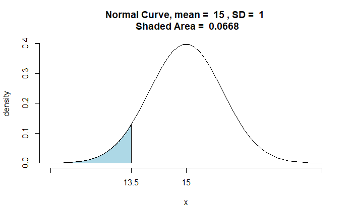
Becky loves running 100-meter races. The run timing for girls her age follows a normal distribution with a mean of 15 seconds and a standard deviation of 1s. The cut-off time to get into the school team is 13.5 seconds. If Becky is on the school running team in 100 meters, what is the probability that she runs below 13 seconds?
Without any other information, we can use the given probability distribution to determine the chance of Becky running under 13 seconds.
Since we know she is in the school team, we can update the probability as per Bayes’ theorem. Let’s use the general formula of Bayes’ theorem here:
The first term in the numerator, P(T|13) = 1 (the probability of someone in the team with a cut-off of 13.5 s, given her timing is less than 13s). We already know the second term, P(13), 0.0228.
The denominator, P(T), is the probability of getting on the team, which is nothing but the chance of running under 13.5 seconds. That is,
If ‘moneyline’ is the term used in American betting, it’s ‘fractional odds’ for the UK. So, for today’s premier league match between Chelsea and Everton, the following are the odds.
Home
Draw
Away
14/19
10/3
19/5
This means that if you bet on home, i.e., Chelsea (the match is played in Chelsea’s backyard) and win, you get a profit of £14 for every £19 placed. In other words, you bet £19 and get back £14+£19 = £33.
As before, let’s estimate the implied probability based on the (fair) expected value assumption. E.V = p x 14 – (1-p) x 19 = 0 14p + 19p – 19 = 0 p = 19/(14 + 19) = 0.576 = 57.6%
As a shortcut: for 14/19, p = 1/[(14+19)/19].
And for the next two Draw: p (10/3) = 1/[(10+3)/3] = 0.231 = 23.1% Away (Everton win): p (19/5) = 1/[(19+5)/5] = 0.208 = 20.8%
As expected, the sum of probabilities is not 100% but 101.5%; the house must win.
We have seen how to interpret the betting odds or moneyline. Take, for example, the NBA odds for one of tonight’s matches.
Team
Moneyline
Washington Wizards
+340
Boston Celtics
-450
If you place $100 on the Wizards, and they win, you get $440, suggesting a profit of $340 upon winning (and you lose $100 if they lose). On the other hand, if you bet $450 on the Celtics, and they win, you get $550 (and a loss of $450 if they lose). Your profit for winning is $100.
Implied probability
Let’s apply the expected value concept to this problem. Let p be the probability of winning the prize upon betting on the Wizards. For this to be a fair gamble, the expected value = p x 340 – (1-p) x 100 = 0 p = 100/440 = 0.227 or 22.7%; this is an implied probability of the bet.
Let q be the probability for the Celtics. the expected value = q x 100 – (1-q) x 450 = 0 q = 450/550 = 0.818 or 81.8%
Suppose you add the two probabilities, p + q = 104.5%. It is more than 100%, suggesting they are not the actual probabilities (fair odds) of winning the (NBA) game. Since the actual win probabilities of teams must add up to 100%, the sum p + q must be lower than that obtained in the expected value calculations. Therefore, at least one of the expected values must be < 0.
104.5% may be understood as putting $104.5 the money at risk to get $100 back. The difference (104.5 – 100)/104.5 is the bookie’s edge built into the bet.
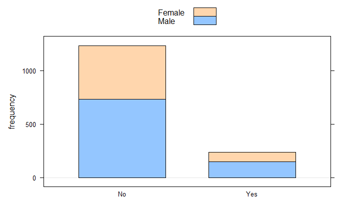
We continue using the ‘tigerstats’ package to analyse the ‘IBM HR Analytics Employee Attrition & Performance’ dataset, a fictional data set created by IBM data scientists and taken from Kaggle. The dataset contains various parameters related to attribution,
         MaritalStatus
Attrition Divorced Married Single
      No       294     589    350
      Yes       33      84    120
xtabs(~Attrition+Gender,data=Em_data)
         Gender
Attrition Female Male
      No     501  732
      Yes     87  150
CIMean
CIMean(~MonthlyIncome,data=Em_data)
ttestGC
ttestGC(~MonthlyIncome,data=Em_data)
Inferential Procedures for One Mean mu:

Descriptive Results:

variable       mean     sd       n
MonthlyIncome  6502.931 4707.957 1470

Inferential Results:

Estimate of mu:	 6503
SE(x.bar):	 122.8

95% Confidence Interval for mu:

          lower.bound         upper.bound
          6262.062872         6743.799713
ttestGC(~Age,data=Em_data)
Inferential Procedures for One Mean mu:

Descriptive Results:

variable  mean     sd       n
Age       36.924   9.135    1470

Inferential Results:

Estimate of mu:	 36.92
SE(x.bar):	 0.2383

95% Confidence Interval for mu:

          lower.bound         upper.bound
          36.456426           37.391193
We have seen how the R package ‘tigerstats’ can help visualise basic statistics. The library has several functions and datasets to teach statistics at an elementary level. We will see a couple of them that enable hypothesis testing.
chi-square test
We start with a test for Independence using the chi-square test. The example is the same as we used previously. Here, we create the database with the following summary.
High School
Bachelors
Masters
Ph.d.
Total
Female
60
54
46
41
201
Male
40
44
53
57
194
Total
100
98
99
98
395
as_tibble(educ)
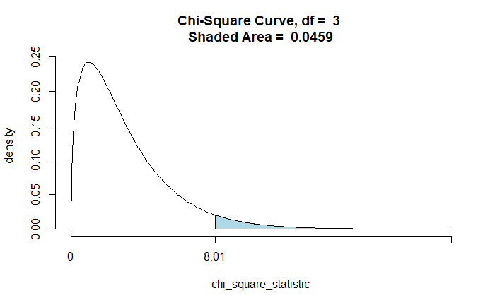
The function to use is ‘chisqtestGC’, which takes two variables (~var1 + var2) to test their association. Additional attributes such as graph and verbose yield the relevant graph (ch-square curve) for the P-value and details of the output.
Pearson's Chi-squared test

Observed Counts:
             SEX
EDU           Female Male
  Bachelors       54   44
  High School     60   40
  Masters         46   53
  Ph.d.           41   57

Counts Expected by Null:
             SEX
EDU           Female  Male
  Bachelors    49.87 48.13
  High School  50.89 49.11
  Masters      50.38 48.62
  Ph.d.        49.87 48.13

Contributions to the chi-square statistic:
             SEX
EDU           Female Male
  Bachelors     0.34 0.35
  High School   1.63 1.69
  Masters       0.38 0.39
  Ph.d.         1.58 1.63


Chi-Square Statistic = 8.0061
Degrees of Freedom of the table = 3
P-Value = 0.0459
Binomial test for proportion
Suppose a coin toss landed on 40 heads in 100 attempts. Perform a two-sided hypothesis test for p = 0.5 as the Null.
binomtestGC(x=40,n=100,p=0.5, alternative = "two.sided", graph = TRUE, conf.level = 0.95)
x = variable under study n = size of the sample p = Null Hypothesis value for population proportion alternative = takes “two.sided”, “less” or “greater” for the computation of the p-value. conf.level = number between 0 and 1, indicating the confidence interval graph = If TRUE, plot graph of p-value
Exact Binomial Procedures for a Single Proportion p:
	Results based on Summary Data

Descriptive Results:  40 successes in 100 trials

Inferential Results:

Estimate of p:	 0.4
SE(p.hat):	 0.049

95% Confidence Interval for p:

          lower.bound         upper.bound
          0.303295            0.502791

Test of Significance:

	H_0:  p = 0.5
	H_a:  p != 0.5

	P-value:		P = 0.0569
binomtestGC(x=40,n=100,p=0.5, alternative = "less", graph = TRUE, conf.level = 0.95)
Exact Binomial Procedures for a Single Proportion p:
	Results based on Summary Data

Descriptive Results:  40 successes in 100 trials

Inferential Results:

Estimate of p:	 0.4
SE(p.hat):	 0.049

95% Confidence Interval for p:

          lower.bound         upper.bound
          0.000000            0.487024

Test of Significance:

	H_0:  p = 0.5
	H_a:  p < 0.5

	P-value:		P = 0.0284
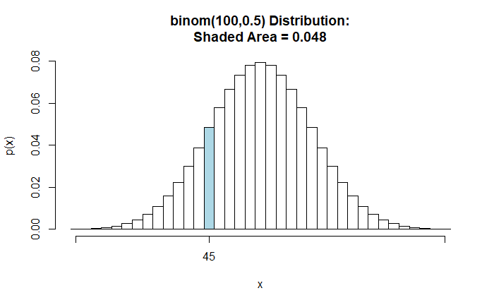
This post refreshes the probability vs likelihood concept and presents a few R functions from the tigerstats library. As usual, we begin with a coin-flipping exercise. What is the probability of obtaining 45 heads upon flipping 100 fair coins? A fair coin is one in which the chance of getting heads equals the chance of getting tails: 0.5.
Coin tossing is a discrete event, and the Y-axis represents the probability. The probability of obtaining 45 heads while flipping 100 fair coins is 0.048.
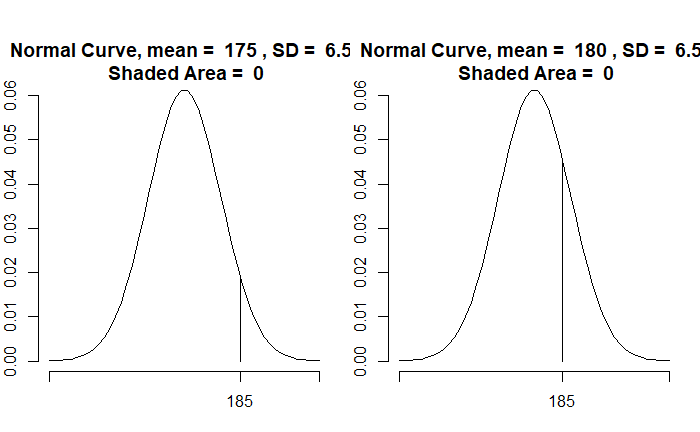
Now, consider a continuous distribution. Suppose the heights of adults are normally distributed in a population with a mean of 175 cm and a standard deviation of 6.5 cm. What is the probability that a random person measures height between 185 and 190 cm?
Notice a few things: the Y-axis is not probability but probability density. The required probability is the area (under the curve) between two values, the height between 185 and 190 cm = 0.0515. In a continuous distribution, where the probability can take every possible value between 0 and 1, getting the chance for precise height (say, 180.0000) does not make sense.
Likelihood
If probability was about getting 45 heads for a coin with p = 0.5 tossed 100 times, the likelihood is the mirror image of that. What is the likelihood of having a fair coin (p = 0.5) if the coin lands 45 heads in 100 tosses?
In likelihood discussions, you have the data, i.e., 45 heads in 100 tosses. The investigator’s task is to find out the coin bias. The likelihood that it’s an unbiased coin (p = 0.5), given that 45 in 100 landed on heads, is 0.048. The likelihood that the coin is biased with p = 0.55, given that 45 in 100 landed on heads, is 0.011. The likelihood that the coin is biased p = 0.4, given that 45 in 100 landed on heads, is 0.048.
Similarly, for heights, The likelihood of a distribution with mean = 175 cm and a standard deviation = 6.5 cm, given the measured height = 185, is 0.019 The likelihood of a distribution with mean = 180 cm and a standard deviation = 6.5 cm, given the measured height = 185, is 0.046
In summary
Probability is about the chance of data under a given distribution, P(Data|Distribution)
Likelihood is about the distribution for the given data, L(Distribution|Data)
The effect of screen time on mental and social well-being is a subject of great concern in child development studies. The common knowledge in the field revolves around the “dispalcement hypothesis”, which says that the harm is directly proportional to the exposure.
Przybylski and Weinstein published a study on this topic in Psychological Science in 2017. The research analysed data collected from 120,115 English adolescents. Mental well-being (the dependent variable) was estimated using the Warwick-Edinburgh Mental Well-Being Scale (WEMWBS ). The WEMWBS is a 14-item scale, each answered on a 1 to 5 scale, ranging from “none of the time” to “all the time.” The fourteen items in WEMWBS are:
1
I’ve been feeling optimistic about the future
2
I’ve been feeling useful
3
I’ve been feeling relaxed
4
I’ve been feeling interested in other people
5
I’ve had energy to spare
6
I’ve been dealing with problems
7
I’ve been thinking clearly
8
I’ve been feeling good about myself
9
I’ve been feeling close to other people
10
I’ve been feeling confident
11
I’ve been able to make up my own mind about things
12
I’ve been feeling love
13
I’ve been interested in new things
14
I’ve been feeling cheerful
The study results
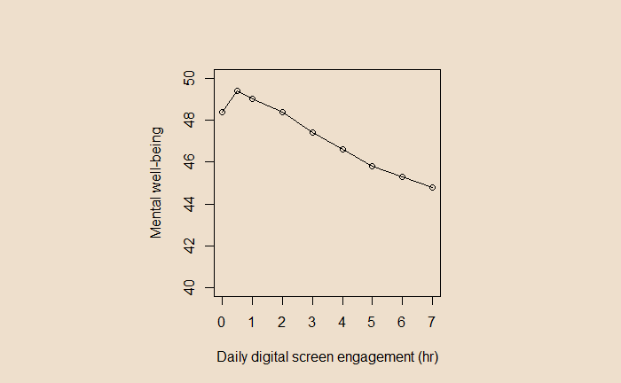
I must say, the authors were not alarmists in their conclusions. The study showed a non-linear relationship between screen time and mental well-being. Well-being increased a bit with screen time but later declined. Yet, the plots were in the following form (see the original paper in the reference for the exact graph).
A casual look at the graph shows a steady decline in mental well-being as the screen time increases from 2 hours onwards. Until you notice the scale of the Y-axis!
In a 14-item survey with a 1-5 range in scale, the overall score must range from 14 (min) to 70 (max). Instead, In the present plot, the scale was from 40 to 50, thus visually exaggerating the impact. Had it been plotted following the (unwritten) rules of visualisation, it would have looked like this:
To conclude
Screen time impacts the mental well-being of adolescents. It increases a bit, followed by a decline. The magnitude of the decrease (from 0 screen time to 7 hr) is about 3 points on a 14-70 point scale.
References
Andrew K. Przybylski and Netta Weinstein, A Large-Scale Test of the Goldilocks Hypothesis: Quantifying the Relations between Digital-Screen Use and the Mental Well-Being of Adolescents, Psychological Science, 2017, Vol. 28(2) 204–215. Joshua Marmara, Daniel Zarate, Jeremy Vassallo, Rhiannon Patten, and Vasileios Stavropoulos, Warwick Edinburgh Mental Well-Being Scale (WEMWBS): measurement invariance across genders and item response theory examination, BMC Psychol. 2022; 10: 31.
In an ordinary linear model, like linear regression exercises, we express the dependant variation (y) as a function of the independent variable (x) as:
The equation is divided into two parts. The first part is the equation of a line.
where beta0 is the intercept and beta1 is the slope of the line. It just described the line (the approximation), but you need to add the error term to include the points around the line. The second part is the error term or the points around the idealised line.
The points around the line are normally distributed in linear regression, so the epsilon term is normal.
LM to GLM
Imagine if the dependent variable is binary—it takes one or zero. The random component (error term) is no longer normally distributed in such cases. That is where the concept of generalised linear models (GLM) comes in. Here, the first part remains the same, while the second part can take other types of distributions as well. In the case of binary, as in logistic regression, GLM is used with binomial distribution through a link function.
link function
random component is a binomial error distribution family.
In Poisson regression, the error term takes a Poisson distribution.
In R, you use glm() with an attribute on the family as, glm(formula, family = “binomial”)
We have seen the use of linear regression models for continuous variables and logistic regression for binary variables. Another class of variables is called count variables, such as,
The number of claims received per month by an insurance company Weekly accidents happening in a particular region
The dependent variables (claims or accidents) in these examples have a few standard features. The data represent numbers (counts) or rates (counts per time). They also can only take values of zero or positive discrete numbers. As the Poisson random variable is used to model counts, the relevant regression in the above examples could be Poisson regression.
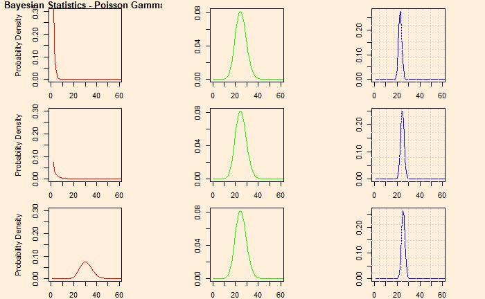
We assume that flight accidents are random and independent. This implies that the likelihood function (the nature of the phenomenon) is likely to follow a Poisson distribution. Let Y be the number of events occurring within the time interval.
Theta is the (unknown) parameter of interest, and y is the data (total of 10 observations). We will use Bayes’ theorem to estimate the posterior distribution p(theta|data) from a prior, p(theta). As we established long ago, we select gamma distribution for the prior (conjugate pair of Poisson).