Data & Statistics

Confidence Interval vs Credible Interval

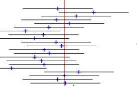
Confidence interval is a frequentist’s way of communicating the range of values within which the actual (population) parameter sits. A confidence interval of 90% implies that if you do 20 random samples from the same target population and with the same sample size, 18 of the confidence intervals cover the true population mean. This is the frequentist’s view, and the parameter is fixed. 

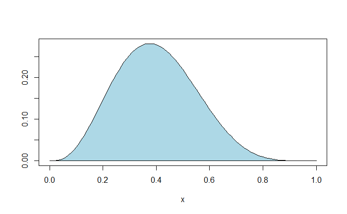
On the other hand, the Bayesian does not have a concept of a fixed parameter and is happy to accept it as an unknown quantity. Instead, she gives a probability distribution to the expected outcome. The range of values (the interval) of the probability distribution (plausibility) is the credibility interval. In a 90% credible interval, the portion of the (posterior) distributions between the two intervals will cover 90% of the area.

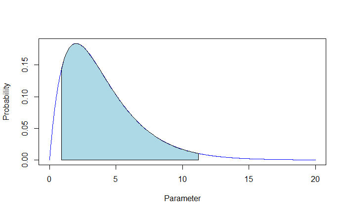
For example, in the following posterior distribution, there is a 90% plausibility that the parameter lies between 0.9 and 11.2; the shaded area = 0.9.

Confidence Interval vs Credible Interval Read More »

Lewis Carroll’s Pillow Problem

Here is one of the Lewis Carroll’s Pillow Problems (problem # 5):

A bag contains a counter, known to be either white or black. A white counter is put in, the bag is shaken, and a counter is drawn out, which proves to be white. What is now the chance of drawing a white counter?

We will use Bayes’ theory to get the required probability.

\\ P(W other|W taken) = \frac{P(W taken|W other) * P(W other)}{P(W taken|W other) * P(W other) + P(W taken|B other) * P(B other)} \\ = \frac{1*1/2}{1*1/2 + 1/2*1/2}

= 1/2/[1/2+1/4] = 2/3 = 0.66

Lewis Carroll’s Pillow Problem Read More »

Bayesian Persuasion

Persuasion is the act of a person (a.k.a. the sender) to convince another (the receiver) to decide in favour of the sender. Suppose the receiver is a judge and the sender is the prosecutor. The prosecutor aims to make the judge convict 100% of the defendants. But the judge knows that only a third of the defendants are guilty. Can the prosecutor persuade the judge to get more than 33% of the decisions in her favour? If the judge is rational, what should be the prosecutor’s strategy?  

Suppose the prosecutor has the research report and the knowledge about the truth. She can follow the following three strategies.

Strategy 1: Always guilty

The prosecutor reports that the defendant is guilty 100% of the time, irrespective of what happened. In this process, the prosecutor loses credibility, and the judge resorts to the prior probability of a person being guilty, which is 33%. The result? Always acquit the defendant. The prosecutor’s incentive is 0. 

Strategy 2: Full information

The prosecutor keeps it simple – report what the research finds. It makes her credibility 100%, and the judge will follow the report, convicting 33% and acquiring 66%. The prosecutor’s incentive is 0.33. 

Strategy 3: Noisy information

Here, when the research suggests the defendant is innocent, report that the defendant is guilty slightly less than 50% of the time and innocent the rest of the time. Let this fraction be 3/7 for guilty and 4/7 for innocent. 

From the judge’s perspective, if she sees an ‘innocent’ report from the prosecutor, she will acquit the defendant. The proportion of time this will happen is (2/3) x (4/7) or 40%. Remember, 2/3 of the defendants are innocent! On the other hand, she will apply the Bayes’ rule if she sees a guilty report. The probability that the defendant is guilty, given the prosecutor provided a guilty report, P(g|G-R), is

P(g|G-R) = P(G-R|g) x P(g) / [P(G-R|g) x P(g) + P(G-R|i) x P(i)]
= 1 x (1/3) /[1 x (1/3) + (3/7) (2/3)]
= (1/3)/(13/21) = 0.54

The judge will convict the defendant since the probability is > 50%. So, the overall conviction rate is 100 – 40 = 60%. The prosecutor’s incentive is 0.6. 

Conclusion

So, persuasion is the act of exploiting the sender’s information edge to influence the receiver’s decision-making. As long as the sender mixes up the flow of information to the judge, she can maximise the decisions in her favour, in this case, from 33% to 60%. 

Emir Kamenica and Matthew Gentzkow, American Economic Review 101 (October 2011): 2590–2615

Bayesian Persuasion Read More »

Response Bias

This type of bias is common in surveys, where the individual’s answer tends to be inaccurate or non-representative of the population. It can significantly impact the research; we will see some common types here. 

Voluntary response bias

The people who responded to the survey differed from the general population due to their personal experience. A typical example is the star rating, in which people with extreme experiences, either highly satisfied or highly unsatisfied, tend to respond more often than those with average experience. 

Social response bias

Also known as the social desirability bias, this bias occurs when individuals choose to respond in a way that makes them look good in front of others. In the end, good behaviour is overreported, and bad behaviour is underreported. 

Non-response bias

Suppose the people who participate in the survey are systematically different from those who don’t. A telephonic survey, say via land phone, is an example that collects only the people available at home during the calling hours. 

Response Bias Read More »

The Rating Problem

Here is the rating summary of a product,
Good – 40%
Average – 10%
Poor – 50%
Looking at the product, how do you know which view represents the actual quality of the product?

Can we conclude that the probability of the product being good equals 0.4, average 0.1, and poor 0.5? Although that is what we want from the rating system, we must realise that these may not represent the absolute or marginal probability of quality but the conditional probability, e.g., the probability of good a given person has rated. In other words

P(Good|Rated) = 0.4
P(Average|Rated) = 0.1
P(Poor|Rated) = 0.5

From this information, we can estimate the actual probabilities, P(Good), P(Average) and P(Poor) using Bayes’ theorem. 

P(Good|Rated) = P(Rated|Good) x P(Good) / P(Rated)
P(Average|Rated) = P(Rated|Average) x P(Average) / P(Rated)
P(Poor|Rated) = P(Rated|Poor) x P(Poor) / P(Rated)

The Rating Problem Read More »

P-Hacking

P-hacking is an often malicious practice in which the analysis is chosen based on what makes the p-value significant. Before going into detail, let’s recall the definition of p-value. It is the probability that an effect is seen purely by chance. In other words, if we chose 5% as the critical p-value to reject (or fail to reject) a null hypothesis, 1 in 20 tests will result in a spectacular finding even when there was none. 

So what happens if the researcher carries out several tests and reports only the one with the ‘shock value’ without mentioning the context of the other non-significant tests? It becomes an example of a p-hacking. 

References

P-Hacking: Crash Course Statistics: CrashCourse
Data dredging: Wiki
The method that can “prove” almost anything: TED-Ed

P-Hacking Read More »

Confusion of the Inverse

What is the safest place to be if you drive a car, closer to home or far away?

Take this statistic: 77.1 per cent of accidents happen 10 miles from drivers’ homes. You can do a Google search on this topic and read several reasons for this observation, ranging from overconfidence to distraction. So, you conclude that driving closer to home is dangerous. 

However, the above statistics are useless if you seek a safe place to drive. Because what you wanted was the probability of an accident, given that you are near or far from home, say P(accident|closer to home). And what you got instead was the probability that you are closer to home, given you have an accident P(closer to home|accident). Look at the two following scenarios. Note that P(closer to home|accident) = 77% in both cases.

Scenario 1: More drive closer to home

Home Away
Accident7723100
No
Accident
10002001200

Here, out of the 1300 people, 1077 drive closer to home.
P(accident|closer to home) = 77/1077 =0.07
P(accident|far from home) = 23/223 = 0.10
Home is safer. 

Scenario 2: More drive far from home

Home Away
Accident7723100
No
Accident
10005001500

Here, out of the 1600 people, 1077 drive closer to home.
P(accident|closer to home) = 77/1077 =0.07
P(accident|far from home) = 23/523 = 0.04
Home is worse 

This is known as the confusion of the inverse, which is a common misinterpretation of conditional probability. The statistics only selected the people who had been in accidents. Not convinced? What will you conclude from the following? Of the few tens of millions of people who died in motor accidents in the last 50 years, only 19 people died during space travel. Does it make space safer to travel than on earth? 

Confusion of the Inverse Read More »

Annie’s Table Game – The End Game

In the last exercise, we found that the frequentist solution heavily underpredicted Becky’s chances of winning the table game. This time, we will see how much that depended on the sample size. So, they continued the game but played 80 matches in total—Annie winning 50 to Becky’s 30. What are Becky’s chances of winning the next three games?

Frequentist solution 

This is not different from the previous: Based on the results, with 30 wins in 80 matches, Beck’s probability of winning a game is (3/8). That means the probability of Becky winning the next three games is (3/8)3 = 0.053.

Bayesian solution 

Run the R program we developed last time:

library(DescTools)
x <- seq(0,1,0.01)
AUC(x, choose(80,30)*x^33*(1-x)^50, from = min(x, na.rm = TRUE), to = max(x, na.rm = TRUE))  /
AUC(x, choose(80,30)*x^30*(1-x)^50, from = min(x, na.rm = TRUE), to = max(x, na.rm = TRUE)) 
0.057

And the Simulations

itr <- 1000000
beck_win <- replicate(itr, {
  beck_pro <- runif(1)
  p_5_3 <- dbinom(30, 80, beck_pro)

  if(runif(1) < p_5_3){
    game_5_3 <- 1
  }else{
    game_5_3 <- 0
  }
  
  
  if(game_5_3 == 1){
     beck_3_0 <- beck_pro^3
  } else{
     beck_3_0 <- 0
  }
  
  
  if(beck_3_0 == 0){
    win_beck <- "no"
  }else if(runif(1) < beck_3_0){
    win_beck <- "Becky"
  }else{
    win_beck <- "Annie"
  }
  
  })

sum(beck_win == "Becky")/(sum(beck_win == "Becky") + sum(beck_win == "Annie"))
0.058

Well, when the number of data points is large, the frequentist solution reaches what was simulated.

Annie’s Table Game – The End Game Read More »

Annie’s Table Game – Frequentist vs Bayesian 

See the story and numerical experiments in the previous post. Annie is currently leading 5-3; what is the probability that Becky will reach six and win the game?

Frequentist solution 

Based on the results so far, 3 wins in 8 matches, Beck’s probability of winning is (3/8). That means the probability of Becky winning the next three games (to reach 6 before Annie wins another, which will make her 6) is (3/8)3 = 0.053.

Bayesian solution 

First, we write down the Bayes equation. The probability of B winning the game, given A is leading 5-3, 

\\ P(B|A_{5-3}) = \frac{P(A_{5-3}|B)*P(B)}{P(A_{5-3})}

Let’s start with the denominator. If p represents the probability of Becky winning a game, the probability of a 3-5 or 3 in 8 result is obtained by applying the binomial equation. The denominator is the sum of all possible scenarios (p values from 0 to 1). In other words, The denominator is,

\\ P(A_{5-3}) = \int_0^1 _8C_3 p^3 (1-p)^5

We use an R shortcut to evaluate the integral as the area under the curve using the ‘AUC’ function from the ‘DescTools’ library.

library(DescTools)
x <- seq(0,1,0.01)
AUC(x, choose(8,3)*x^3*(1-x)^5, from = min(x, na.rm = TRUE), to = max(x, na.rm = TRUE)) 
0.1111

And here is the area. 

plot(x, choose(8,3)*x^3*(1-x)^5, type="l", col="blue", ylab = "")
polygon(x, choose(8,3)*x^3*(1-x)^5, col = "lightblue")

The numerator is the multiplication of the likelihood function with the prior probability of Becky winning three games. We will use a binomial equation as the prior function and p x p x p = p3 as P(B). 

\\ P(A_{5-3}|B)*P(B) = 8C_3 p^3 (1-p)^5 p^3 \\ \\ 8C_3 p^6 (1-p)^5

Again, the area under the curve all possible p values (0 -1),

AUC(x, choose(8,3)*x^6*(1-x)^5, from = min(x, na.rm = TRUE), to = max(x, na.rm = TRUE)) 
0.0101

The required Bayesian posterior is 0.0101/0.1111 = 0.0909

To sum up

The Bayesian estimate is almost double compared to the frequentist. The Bayesian estimate is much closer to the results we saw earlier. Does this make Bayesian the true winner? We’ll see next. 

Annie’s Table Game – Frequentist vs Bayesian  Read More »

Annie’s Table Game

Annie and Becky are playing a game in which the aim is to secure six points first. The Casino randomly rolls a ball onto the table, and the point at which the ball rests is marked. The Casino then rolls another ball at random. If it comes to rest to the left of the initial mark, Annie wins the point; to the right, Becky wins. If Annie is currently leading 5-3, what is the probability that Becky will win the game?

Before we get into statistical methods, we will play the game a million times using R. 

First step: Becky’s chance of winning any game is a random number with uniform probability. If that is the case, the probability of Annie leading 5-3 (or Becky winning 3 out of 8 games) is given by binomial distribution.

beck_pro <- runif(1)
p_5_3 <- dbinom(3, 8, beck_pro)

That gives the probability of having a 5-3 lead for Annie, but that doesn’t mean it will happen for sure. For that to happen, the estimated probability must be greater than a random number between 0 and 1.

  if(runif(1) < p_5_3){
    game_5_3 <- 1
  }else{
    game_5_3 <- 0
  }

Thus, we established instances where Annie was leading 5-3. We will estimate the probability of Becky winning the next three games. 

  if(game_5_3 == 1){
     beck_3_0 <- beck_pro^3
  } else{
     beck_3_0 <- 0
  }

Like we did before, a random number is generated, and if it is less than the probability of Becky winning the next three games, Becky wins; otherwise, Annie wins. 

 if(beck_3_0 == 0){
    win_beck <- "no"
  }else if(runif(1) < beck_3_0){
    win_beck <- "Becky"
  }else{
    win_beck <- "Annie"
  }
  
  })

Calculate this a million times and estimate the proportion of Becky’s win over total wins.

itr <- 1000000
beck_win <- replicate(itr, {
  beck_pro <- runif(1)
  p_5_3 <- dbinom(3, 8, beck_pro)

  if(runif(1) < p_5_3){
    game_5_3 <- 1
  }else{
    game_5_3 <- 0
  }
  
  
  if(game_5_3 == 1){
     beck_3_0 <- beck_pro^3
  } else{
     beck_3_0 <- 0
  }
  
  
  if(beck_3_0 == 0){
    win_beck <- "no"
  }else if(runif(1) < beck_3_0){
    win_beck <- "Becky"
  }else{
    win_beck <- "Annie"
  }
  
  })

sum(beck_win == "Becky")/(sum(beck_win == "Becky") + sum(beck_win == "Annie"))
0.09057296

Introduction to Bayesian Statistics – A Beginner’s Guide: Woody Lewenstein

What is Bayesian statistics?: Nature Biotechnology,  volume 22, 177–1178 (2004)

Annie’s Table Game Read More »