Data & Statistics

Shaq Goes to the White House

Shaquille O’Neil, popularly known as Shaq, is a basketball player and four-time NBA champion. He once had a bet with his friend about getting into the White House without prior permission. The wager was 1000 push-ups.

What is the chance of Shaq to be successful?

We can use binomial probability mass function (PMF) to estimate Shaq’s chance.

f(s; n,p) = \binom{n}{s} p^s (1-p)^{n-s}

Where n is the number of trials, s is the number of successes, and p is the probability of success.

Since Shaq was confident to bet, one can imagine that he would have given a higher value of p (say 0.9) for himself, whereas his friend would think lower (say, 0.2). If Shaq has one chance to show up, called a Bernoulli trial, associated probabilities with those two conditions are:

\\ f(1; 1,0.9) = \binom{1}{1} 0.9^1 (1-0.9)^{1-1} = 0.9 \text { and} \\ \\    f(1; 1,0.2) = \binom{1}{1} 0.2^1 (1-0.2)^{1-1} = 0.2

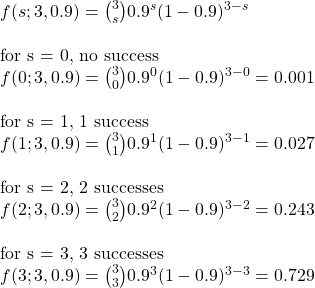
If Shaq makes three attempts, as per his view, the success rates are:

\\ f(s; 3,0.9) = \binom{3}{s} 0.9^s (1-0.9)^{3-s} \\ \\ \text{for s = 0, no success} \\ f(0; 3,0.9) = \binom{3}{0} 0.9^0 (1-0.9)^{3-0} = 0.001 \\ \\ \text{for s = 1, 1 success} \\ f(1; 3,0.9) = \binom{3}{1} 0.9^1 (1-0.9)^{3-1} = 0.027 \\ \\ \text{for s = 2, 2 successes} \\ f(2; 3,0.9) = \binom{3}{2} 0.9^2 (1-0.9)^{3-2} = 0.243 \\ \\ \text{for s = 3, 3 successes} \\ f(3; 3,0.9) = \binom{3}{3} 0.9^3 (1-0.9)^{3-3} = 0.729

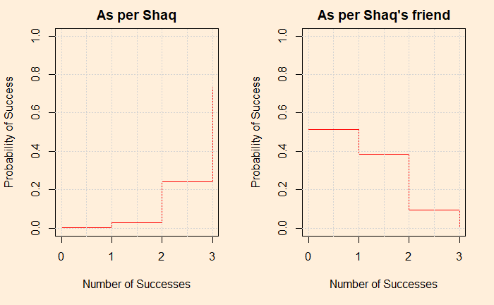
The probability densities for Shaq and his friend, in graphical format, are:

Was Shaq successful?

No, he was not. He tried once but was stopped at the gate by the security! What would have happened had he made another attempt? More about that story and the use of Baysian in the next post.

Shaq Denied Entrance: Washington Post

Shaq Goes to the White House Read More »

Has UK Weathered the Storm?

This post follows up on the one made in December. Covid’s latest variant, the omicron, was a storm that played havoc over the world. The actual calamity is not known yet, but there is a widespread feeling that it was milder.

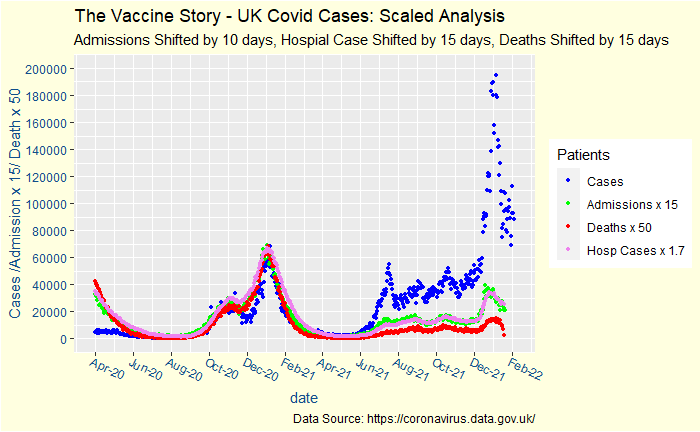
The UK, one of the countries that captured and shared covid data from day 1, provides answers to some of those questions. Here is an update of what happened since last time. Note the deaths of the last few days are incomplete.

Critical parameters such as hospitalisations and deaths have been rescaled – both x and y axes – to coincide with the reported cases before the vaccine.

Has UK Weathered the Storm? Read More »

Who Wrote paper No. 54?

The Federalist papers were published anonymously in 1787-88 by Alexander Hamilton, John Jay and James Madison. Of the 77 essays, it is generally agreed that Jay wrote 5, Hamilton 43 and Madison 14. The remaining papers are either jointly written by Hamilton and Madison or by one of the two (not Jay). The problem was solved by Mosteller and Wallace using the Bayesian approach but using Poisson distribution.

We try to go through their approach using a simple Bayes’ rule. Consider paper no. 54. The starting point was the style of writing. Both Hamilton and Madison used similar styles, so it was difficult to get an answer that easily. The authors then looked for the usage of specific words, such as by, from, to, while, whilst, war etc. We take one such word, upon. The frequency distribution of upon collected from a set of papers published by Hamiton and Madison (including the ones outside The Federalist) is given below

Rate / 1000HM
0041
(0,1]17
(1,2]102
(2,3]11
(3,4]11
(4,5]10
(5,6]3
(6,7]1
(7,8]1
Total4850

Bayesian Problem

Let’s the formula the problem using upon as the tag word:
In paper 54, the word upon comes 2 times in the text (in 2004 words). So upon frequency is 0.99.
P(Hamilton|upon = 0.99) = P(upon = 0.99|Hamilton) * P(Hamilton) / [P(upon = 0.99|Hamilton) * (Hamilton) + P(upon = 0.99|Madison) * P(Madison)]

P(upon = 0.99|Hamilton) = (1/48) based on the frequency table
P(upon = 0.99|Madison) = (7/50) based on the frequency table
P(Hamilton) = can be 43/77 based on the existing known data of authorship. But we take 0.5
P(Madison) = can be 14/77 based on the existing known data of authorship. But we take 0.5

P(Hamilton|upon = 0.99 ) = (1/48 * 0.5)/(1/48 * 0.5 + 7/50*0.5) = 0.13 or 13%. Naturally, P(Madison|upon = 0.99) = 1 – P(Hamilton|upon = 0.99) = 87%

The Federalist Papers: No. 54

Inference in an Authorship Problem: Mosteller and Wallance, Journal of American Statistical Association, 58 (302), 275-309

Who Wrote paper No. 54? Read More »

Back to basics

In the beginning, there was dice

Probability on the margins

dice, game, random-1963300.jpg

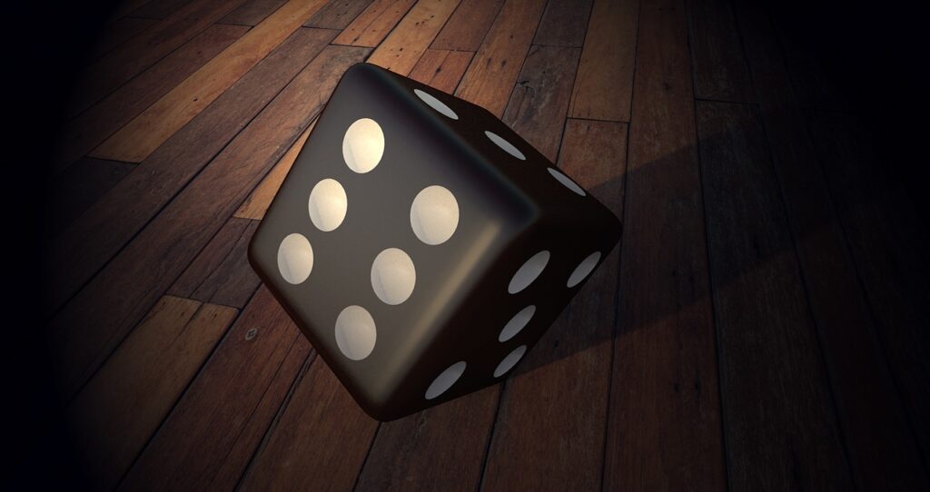
What is the probability of getting a 3 on a single roll of dice? You can calculate that by dividing the number of 3s by all possible numbers the die has.

123456

It is one 3 out of the possible six numbers, or (1/6). The probability of this type is called a marginal probability. The probability of one character of interest, say P(A). Or the one that is on the margins!

Two things at once

dice, die, cube-149215.jpg

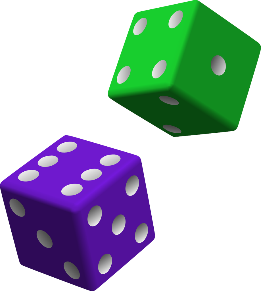
You throw two dice – one green and one violet. What is the probability that you get a green 3? It is the joint probability of two outcomes – a colour and a number – at once. The notation is:

P(Green \displaystyle \cap 3)

The upside-down U is the symbol of intersection or AND.

Green 1Green 2Green 3Green 4Green 5Green 6
Violet 1Violet 2Violet 3Violet 4Violet 5Violet 6

Only one instance of Green 3 in a total of possible 12 outcomes, so the joint probability is (1/12). When you hear joint, imagine an upside-down U and think it meant AND. What about the opposite?

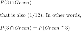
\\ P(3 \displaystyle \cap Green)  \\ \\ \text{that is also (1/12). In other words,} \\ \\ P(3 \displaystyle \cap Green)  = P(Green \displaystyle \cap 3)

Two things, with a clue

Now, what is the probability of seeing a 3 given it is a Green? This is a conditional probability and is represented as:

P(3 | Green)

You don’t need another table to answer that. If green is known, then there is only 1 out of 6 chances for a 3 or (1/6). What about the opposite, P(Green|3)? It’s (1/2) because if 3 is known, the choices are only two: green or violet. So, remember, P(A|B) and P(B|A) are not equal.

Formalising

We will start with the definition of joint probability as we had seen in AND rule earlier.

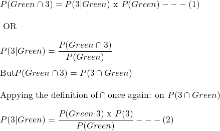
\\ P(Green \displaystyle \cap 3) =P(3 | Green) \text{ x }  P(Green)  --- (1) \\ \\ \text{   OR} \\ \\ P(3 | Green) = \frac{P(Green \displaystyle \cap 3)}{P(Green)}   \\ \\ \text{But} P(Green \displaystyle \cap 3) = P(3 \displaystyle \cap Green) \\ \\  \text{Appying the definition of}  \displaystyle \cap \text{once again: on } P(3 \displaystyle \cap Green) \\ \\ P(3 | Green) =  \frac{P(Green| 3) \text{ x } P(3)}{P(Green)}   --- (2)

Does the last equation remind you of something? Yes, it is one form of Bayes’ equation.

Let’s verify with numbers: first, equation (1) P(Green AND 3) = P(3|Green) x P(Green) = (1/6)x(1/2) = (1/12). Equation (2) P(3|Green) = P(Green|3) x P(3)/ P(Green) = (1/2) x (1/6) / (1/2) = (1/6).

The dice example is simplistic because the descriptors Green and 3 are independent. It’s fun once we have more dependent probabilities. But then, we have seen many of them in the previous posts.

Bayes’ equation

Look at the equation again.

P(3 | Green) =  \frac{P(Green| 3) \text{ x } P(3)}{P(Green)}

  1. The equation relates P(3|Green) with P(Green|3)
  2. The equation calculates P(3) from a known value of P(3)! Don’t you see P(3) on both sides? In case you don’t, P(3|Green) is, after all, P(3). The difference is that some additional information in the name of green is available to use. It is still about P(3) and not about P(Green). So to rephrase observation 2, the Bayes’ equation updates the knowledge of P(3) using additional information. That additional information comes from P(Green).

Back to basics Read More »

The Probability of 100 posts

Reaching one hundred days is a milestone. The general focus of my posts over these days, and also likely in the near future, has been about understanding risks, differentiating them from perceived risks and making decisions in situations of uncertainty using prior information, also known as Bayesian thinking. It started from the misery of seeing how the responsible agents of society -journalists, the political leadership, or whoever influences the public – ignore critical thinking and present a distorted view of reality.

Probability and evolution

A subplot that is closely associated with probability and randomness is the topic of evolutionary biology. It is hard to comprehend, yet the truth about life is that it moved from one juncture to another through chance. Evolution is misleading if you view the probability from hindsight. Changes happen through random errors, but one at a time, so that every step in the process is a high-probability event. Indeed, getting an error at a specified location during the body’s 30 trillion cell divisions is close to zero, but getting one at an unspecified somewhere is close to one. In other words, the designer has deeper trouble explaining a move than a drunken gambler!

Biases and fallacies

Next up is our biases and fallacies. The title of this post already suggests two of them – survivorship bias and the fallacy of hindsight. The probability of delivering an uninterrupted string of 100 articles in 100 days is small, and I would never have chosen the present title had I missed a post on one of these days. Now that it happened (luck, effort or something else), I claim I’ve accomplished a low-probability event. As long as I have the power to change the blog title until the last minute, I am fine. But scheduling a post today, for 100 days from now, with a caption of 200 days, is risky and, therefore, not a wise thing to do if you are risk-averse.

Deteminism or probability

Why does the subject of probability matter so much when we can understand physical processes in a deterministic sense? We grew up in a deterministic world, i.e. a world that taught us about actions and reactions, causes and effects. However, we also deal with situations where the outcomes are uncertain, which is the realm of probability. The impact of lifestyle on health, growth of wealth in the market, action of viruses on people with varying levels of immunity, the possibility of earthquakes, droughts, the list is endless. You can argue that the complexity of variables and the gaps in the understanding demand stochastic reasoning.

Updation of knowledge and Bayesian thinking

However imperfect it may be, Bayesian thinking is second nature to us. You are watching an NBA match in the last seconds, and your team is trailing by a point. Your team gets two free throws. What is in your mind when Steph Curry comes in for those? Contrast that with Ben Simmons. It is intuitive Bayesian thinking. It is not a surprise that you are more at ease with Curry’s 91% success rate in free throws than Ben, who is at 60%. You may not remember those numbers, but you know it from gut feeling.

Yet, being rational requires constant training. Your innate Baysian is too vulnerable to biases and fallacies. You start missing the base rates, confuse the hypothesis given the evidence with evidence given the hypothesis, or overestimate the prior due to recency bias. Surviving the sea of probability is hard, fighting the wind of lies and the sirens of misinformation. So what do you prefer, put wax in the ears, tie tight to the mast or get the rational power, listen to the music, and persist the voyage?

The Probability of 100 posts Read More »

The Heuristics Fight Back

This post supports heuristics as a practical tool for decision making. The proponents of heuristics score a few points when it comes to managing firefighting situations or dealing with the world of randomness, where a deep subject knowledge offers no added advantage. Heuristics suffer from shortcomings that prevent them from helping the world pull out from its biases and fallacies. I will end this article with some observations that I found in the book by Gigerenzer et al.

What is Heuristics?

It is a method of solving practical problems without using extensive rational knowledge. While it is not random guesswork, it can be closer to making educated guesses. It uses the characteristic evolutionary traits of our species in responding to external stimuli. One popular book which comes closer to this description is Blink by Malcolm Gladwell.

Claims of Heuristics

Heuristics claims superior decision quality with a minimum amount of information. They frequently use the adjectives such as simple, practical, minimalist to describe the technique. I will focus on the book of Gigerenzer et al. in the rest of the post. The book is titled, The Simple Heuristics That Make Us Smart.

Toolkits and Workflows

The book opens with an example of managing heart attack victims with the help of a simple checklist. What you see in the list are a few simple questions. They included noting the patient’s systolic blood pressure, age, and heartbeats. Follow this short and sweet classification hierarchy, and you just made a decision.

The book conveniently ignores the origin of how those few vital parameters ended up on the list and what type of history-matching (not the so-called experience) done to those parameters. In other words, the checklist is not something the specialist made up at that moment, however appealing that thought could be. And it doesn’t ignore any quantitative information as the authors appear to claim. Each of the questions in the checklist suggests something about prior knowledge (data), the pillar of Bayesian thinking. It is like claiming pre-cooked meals as an invention to replace a complex cooking process. It is just an illusion to the customer; someone (or a machine) needed to cook somewhere.

Appeal to authority and Appeal to emotions

It is no coincidence that the authors fell into the trap that has been the main criticism against the heuristics – that they can not avoid logical fallacies. The first page itself gives two examples. Starting with a quote attributed to Isaac Newton:

Truth is ever to be found in simplicity, and not in the multiplicity and confusion of things.

Then comes the opening sentence:

A man is rushed to a hospital in the throes of a heart attack. The doctor needs to decide quickly whether the victim should be treated as a low-risk or a high-risk patient.

Simple Heuristics That Make Us Smart, Gerd Gigerenzer, Peter M. Todd, and the ABC Research Group

The subject did not require either of the two quoted statements to prove its point. Heuristics is a practical recipe in decision making.

Final verdict 

The book’s proposal to replace the first revolution (computing probabilities etc.) with the second one (adaptive toolbox with fast and frugal heuristics) is rejected! It is pure short-sightedness. Instead of abandoning probability, the alternative proposal may be to promote heuristics as a practical tool. And working side by side with its older sister is no shame.

The quote, “Truth is ever found …” is utter nonsense; sounds nice but far from the truth!

The Heuristics Fight Back Read More »

The problem with Experience

Imagine this: a peaceful city of a million population wakes up with news of a murder. Its inhabitants, not used to such events, naturally get shocked and think of it as a failure of the establishment. The administration recruits a highly specialised cop from an area of another city notorious for criminals. The place was in such a bad shape that it had 10000 people and 100 criminals, and the officer had a lot of experience catching them.

The cop knows the strength of facial recognition systems as he had a high success rate in catching criminals in his old job. He trusts it was because of the high accuracy of the system, i.e. a 1% false-positive rate and a 100% true positivity (if you are a criminal, you are caught). Is recruiting the top cop a good strategy?

The answer depends on how much of the previous experience the cop was willing to forget and learn the reality of the new city. Look at, mathematically, the problem with his background. We use Bayes’ theorem.

Violent City: prevelance of criminal P(C) = 100/10000 = 0.01, P(+ve|C) = 1, P(+ve|nC) = 0.01, P(nc) = 1 – P(C). Chance of the person is a criminal given the facial recognition is matched, P(C|+ve) = (1 x 0.01) / [1 x 0.01 + 0.01 x 0.99] = 0.5 = 50%; he was right half the time.

Peaceful City: prevelance of criminal P(C) = 100/1000000 = 0.0001, P(+ve|C) = 1, P(+ve|nC) = 0.01, P(nc) = 1 – P(C). P(C|+ve) = (1 x 0.0001) / [1 x 0.0001 + 0.01 x 0.9999] = 0.01 = 1%.

The right level of experience

If the officer uses his experience and starts using a facial recognition system to randomly check people, expect him to catch 99 innocent for every potential criminal. Instead, he can use the tool as supporting evidence for those who are caught for other suspicious activities.

Now replace murder with drinking, facial recognition with a breath analyser. The results will be the same as long as the tool is employed for random checking – a lot of innocents are penalised.

The problem with Experience Read More »

The Fallacy of the Inverse

Let us start from where we ended yesterday, the P -> Q problem. Remember the truth table?

PQP -> Q
truetruetrue
truefalsefalse
falsetruetrue
falsefalsetrue

The way to read the truth table is:

If P is true, Q has to be true. It is called direct reasoning. Q false with P true is a violation of the rule, and therefore if Q is false, P has to be false (indirect reasoning). Finally, if P is not true, Q can be true or false. 

Re-look at the earlier rain problem – if it rains, I will take an umbrella. The only thing that is not possible is rain and no umbrella. The statement, it doesn’t rain now, and therefore, I should not have an umbrella [1] is not true; I can have an umbrella, whether it rains or not. Also, the statement, I am carrying an umbrella, and therefore it is raining [2] is also wrong.

The above statements numbered 1 and 2 mark two widespread logical errors. [1] is called the fallacy of the inverse. An example is: if it’s a dog, it has a tail. The fallacy is if it is not a dog, it can not have a tail. But what about a cat?

[2] is called the fallacy of the converse. An example is catholic priests are men. He is a man and, therefore, must be a catholic priest.

From the examples so far, it seems the inverse and converse errors are easy to spot and escape; until you reach more complex situations such as the equation of life! Yes, the Bayesian way of interpreting evidence. Take our famous example, suppose the probability of having a test is positive given the person has the disease (sensitivity of the equipment) is 95% or P(+|D). We know from our earlier discussions that this is just one variable in the equation. We need more data to estimate our ultimate quest, i.e. P(D|+) or the probability of having the disease given the test is positive. Yet, most people jump to conclude that the probability of getting the disease is 95%. Let’s re-phrase the equation to the PQ format. If the person has the disease, there is a 95% chance that the instrument will test +ve (P ->Q). But, the public presumes the converse, i.e. the device has tested +ve, and therefore the person has a 95% chance of having the disease, which is utter nonsense for a rare disease (low prior).

Rules of Inference

The Fallacy of the Inverse Read More »

Simpson’s Paradox

Continue on the life of asymmetry. Following is the summary statistics of the admission data at Cambridge in 1996 in science, technology, engineering and mathematics (STEM). What is your conclusion?

Accepted
(women)
Accepted
(men)
Total274584

It doesn’t look good, isn’t it? A clear case of gender discrimination. Now, look at the data further.

Applied
(women)
Accepted
(women)
%Applied
(men)
Accepted
(men)
%
Total118427423.1247058423.6

No real difference in the percentage accepted.

Go further deep

Applied
(women)
Accepted
(women)
%Applied
(men)
Accepted
(men)
%
Computer
Science
267272285825
Economics240632651211222
Engineering164523297225226
Medicine416992457814024
Veterinary
Medi cine
33853161802212
Total118427423247058424

Now, this is interesting! Every department accepted a higher proportion of women who applied, yet the overall percentage favoured men. Known as Simpson’s paradox, this reversal of interpretation after accounting for confounding factors is something we should always pay attention to. In this case, women preferred more competitive departments with lower acceptance rates, whereas more men opted for engineering, which had better acceptance rates.

Simpson’s Paradox Read More »

It’s not (about) flu, mate

Ever since the pandemic started in early 2020, one thing that polarised society was the severity of covid19. On one extreme were people who panicked over getting infected, and on the other were people who considered it as another spell of flu. What is the truth? Now that we have loads of data, it should be easier to find it out.

What is risk?

There are multiple definitions for the word risk. One of them, more technical, we have seen earlier. It is the product of the likelihood of something to happen and the consequence. The second one is from the oxford learner’s dictionary. The possibility of something bad happening at some time in the future; a situation that could be dangerous or have a bad result.

Who was right?

At the moment, both parties had reasons to believe in what they thought – it was risky to some and not to others. In other words, the risk was not the same for everybody. Look at the wealth of data collected by the CDC on cases in the US.

Age
group
Total18-2940-4950-6465-7475-8485+
% in population10016.412.319.29.64.92
% infected10021.714.418.56.73.31.7
% died1000.8417.622.12627.7
population
(estimated)
33054.140.663.431.716.26.6
no of infected (mln)
(estimated)
7015.210.1134.72.31.2
no of deaths
(estimated)
0.850.0070.0340.150.190.220.23
infection rate
(%)
21.228.124.820.414.814.318
death rate!
(%)
0.260.010.090.250.61.33.3
death/death18-29
(any)
171947109284
death/death18-29
(infected)
17.52690213441
! The death rate is not the case fatality rate, it is the actual death rate in the population due to covid

Risks are not equal. Take some absolute numbers: the chance of someone dying of covid 19 (entire 2020-21) was about 0.25%. That doesn’t tell the whole story – for an 85-year-old, it is 3.3%. Another way is to calculate the chance of dying after getting infected. Overall it is ca. 1.2%, but for an 85+, it is ca. 20%!

Another type of risk estimate is relative to a younger age group. The relative risk is ca. 300 for an 85+ (any) of dying of covid, whereas once infected, the relative risk of dying is ca. 450.

You are wrong, it’s not flu

Society is connected. Calculating risks based on the least-risky age group is not the way to understand a contagious disease. Once a least-risky person comes home (or a care home), he has every chance of passing it to elders, whose risk was at least two orders of magnitude higher than the giver. For a modern society based on care-for-others, this is not a behaviour to be proud of.

Infectious diseases will come and go. Scientists will also find out cures for present and future pandemics. But, what is sure to remain untreated is human irrationality and ignorance of risks and asymmetry of life.

Demographic trends of cases and death: CDC

Trends in cases: CDC

Risk of Covid19: CDC

It’s not (about) flu, mate Read More »