Prosecutors fallacy

We have seen that Bayes’ theorem is a fundamental tool to validate our beliefs about an event after seeing a piece of evidence. Importantly, it utilises existing statistics or prior knowledge to get to a conclusion. In other words, our hypothesis gets better representativeness by using Bayes’ theorem.

Take some examples. What are the chances that I have a specific disease, given that the test is positive? How good are my perceptions of a person’s job or abilities just by observing a set of personality traits? What are the chances that the accused is guilty, given that a piece of evidence is against her?

Validating hypotheses based on the available evidence is fundamental to investigations but is way harder than they appear, partly because of the illusion of the mind that confuses the required conditional probability with the opposite. In other words, what we wanted to find is a validation of the hypothesis given the evidence, but what we see around us is the chance of evidence if the hypothesis is true, because often, the latter is part of common knowledge.

To remind you of the mathematical form of Bayes’ theorem
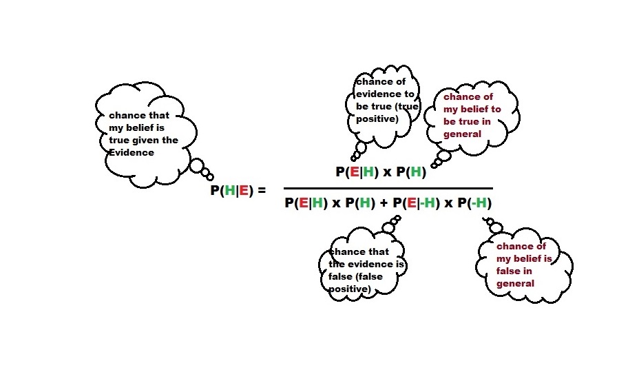
Note that the denominator on the right-hand side is the probability of the evidence P(E)

Confusion between P(H|E) and P(E|H)

What about this? It is common knowledge that a running nose happens if you have a cold. Once that pattern is wired to our mind, the next time when you get a running nose, you assume that you got a cold. If the common cold is rare in your location, as per Bayes’ theorem, the assumption that you made require some serious validation.

Life is OK as long as our fallacies stop at such innocuous examples. But what if that happens from a judge, hearing the murder case? It is the classic prosecutor’s fallacy in which the size of the uncertainty of a test against the suspect is mistaken as the probability of that person’s innocence.

chances of crime, given the evidence = chance of evidence, given crime x (chance of crime/chance of evidence). Think about it, we will go through the details in another post. 

Prosecutors fallacy Read More »
Down Syndrome and Mistakes of Reasoning

We have debunked the mystery of covid infection among the vaccinated population in one of the earlier posts. Today we will see something similar but perhaps far easier to understand.

It is well-known that the risk of Down Syndrome increases with maternal age. For example, women above 40 risk about 11 times higher than those younger than 35 to have babies with Down Syndrome.

Yet, 52% of the mothers who give birth to children with Down Syndrome are 35 years or younger? Based on the data collected from 10 US states and the department of defence between 2006-2010, of the total number of 5600 live births, mothers of 2935 children were women younger than 35.

How did that happen? The simple answer is there were more mothers younger than 35! In the same population set, a whopping 3.7 million out of a total of 4.4 million were mothers below 35!

Small Fractions of Large Numbers

When the number of individuals in the less-risky category becomes very large, the absolute numbers of events also go up, despite its small relative chances to occur. For the vaccination case, the more the percentage of people get vaccinated, the more the absolute number of infected people from the vaccinated category if the society has a high prevalence of infection, which, in turn, is driven by the unvaccinated! But that is temporary – more people getting into the vaccination pool eventually steers the incidence rates down, slowly but steadily.

Selected Birth Defects Data from Population-Based Birth Defects Surveillance Programs in the United States, 2006 to 2010

Epidemiology Visualized: The Prosecutor’s Fallacy

Down Syndrome and Mistakes of Reasoning Read More »

The Big Short and The Assumption of Independence

In the last post, we have seen how banks make money by lending. To get estimates of profits and probabilities, we have assumed two conditions – independence and randomness. This time we look at cases where both these assumptions don’t hold.

Our bank is now making about 1.8 million annual returns with 2000 customers, who have been handpicked for their high credit scores and predictability to repay.

Want for More

An idea was proposed to the management to expand the firm and to increase the customer base. The argument was that even though adding more customers can reduce the predictability of defaulting, the risks could be managed by raising the interest rate a bit higher. Assurance was given that even for an assumed default rate of 5%, which is double the existing, by increasing the interest rate to 6.3%, the bank can make up about 8 million with 99% confidence. She has rationalised her calculations based on the law of large numbers, that the bank is unlikely to miss the target.

The expected value of profit = [interest rate x profit per loan x (1-default rate) – cost per foreclosure x default rate] x total number of loans.

For 20,000 loans, this will mean

[0.063 x 9000 x (1-0.05) – 100,000 x (0.05)] x 20,000

an earning of about 8 millions!

She further shows a plot of the simulation to support her arguments.

It convinced the management, and the company is now on an aggressive lending campaign. The firm has now 20,000 customers and makes a lot of money. A few months later comes a global financial crisis, and the firm is now bankrupt.

Assumption of Independence

To understand what happened to the bank, we should challenge the assumptions used in the original statistical calculations, especially the independence of variables – that one person defaults does not depend on the other. When there are many borrowers with varying capacities to repay, such crises prove detrimental to the business.

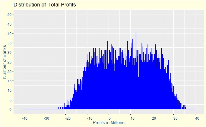
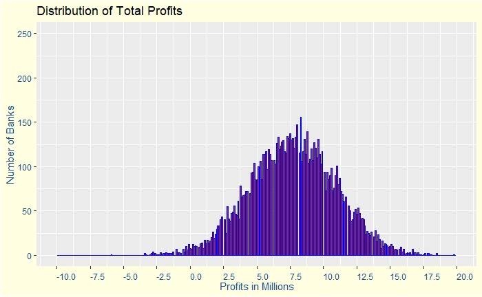
Assume a 50:50 chance, up or down, for everyone to default by a tiny fraction + / – 0.01 (1%) or between 0.04 and 0.06. Note that the average risk of default is still 5% but are no longer independent. Subsequently, the overall chances for making a loss has moved from 1% to 31%, but the average return is still around 8 million. A plot of the distribution of profits is below.

The plot is far from a uniform distribution as the central limit theorem would have predicted using an assumption of complete independence of variables.

The Big Short and The Assumption of Independence Read More »

Interest Rates and How not to Lose Money

In the previous post, we have seen how banks can lose money when they do the business of making money by disbursing loans. This time we will see how banks manage that risk by setting an interest rate for every loan they give. It means every lender needs to pay a fixed proportion of the borrowed money to the bank as a fee.

How does a bank set an internet rate? It is a balance between two opposing forces. If the rate is too low, it will not adequately cover the risk of defaults, and if it is too high, it could keep the customers away from taking loans.

Take the case of 10,000 banks each lends 90,000 dollars per customer to 2000 customers. Let’s say the bank sets an interest rate of 3% on the loans. After running Monte Carlo simulations, we can see the following.
The bank can earn a net profit of about 0.26 mln, but there is a 35% that it will lose money. In other words, 3500 banks won’t make money. The plot below describes this scenario.

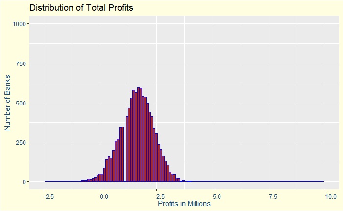
Increase the interest rate to 3.8%. The expected profit is 1.6 mln, and there is about 1% of losing money. That sounds reasonable for a person to run the business. See below for the distribution.


Increase the interest rate to 5% and the profit if we manage to have all the customers intact is 3.77 mln and almost 0% chance of losing money. But a higher interest rate can drive customers away from this bank. Suppose three fourth of the customers have gone to other banks. The profit from 500 customers is less than a million and also there about 0.8% of losing money. Note that fluctuations increase to our estimations – net profits and the chances of making money – as the numbers are smaller (the opposite of the law of large numbers).

Interest Rates and How not to Lose Money Read More »

The Central Limit Theorem

The Central Limit Theorem (CLT). It has intrigued me for a long time. The theorem concerns independent random variables, but it is not about the distribution of random variables. We know that a plot of independent random variables will be everywhere and should not possess any specific pattern. The central limit theorem is about the distribution of their sums. Remember this.

Let us take banks and defaulters to prove this point. Suppose a bank gives away 2000 loans. The bank knows that about 2.5% of the borrowers could default but does not know who those 50 individuals are! That means the defaulters are random. They are also independent. These are two highly debatable notions; once in a blue moon, these assumptions will prove to be the bank’s end. But we’ll deal with it later.

So, what is the distribution of losses to this bank due to defaults? Before that, why is it a distribution and not a fixed number, say, 50 times the loss per foreclosure? Or if the loss per foreclosure is 100,000 per loan, the total loss is 50 x 100,000 = 5 million. A fixed number. That is because a 2.5% default rate is a probability of defaulting, not a certainty. If it is a probability, the total loss to the bank is not a fixed amount but a set of random numbers.

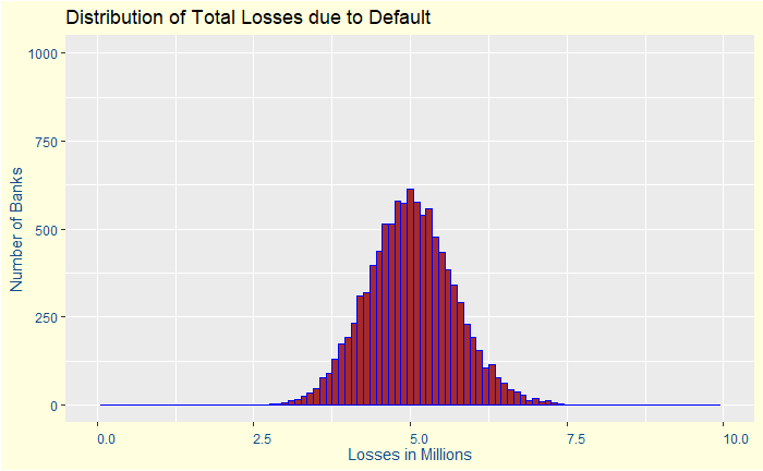
Let’s disburse 2000 loans to people and collect data from 10,000 banks worldwide! How do we do it? By Monte Carlo simulations. The outcome is given below as a plot.

This is the Central Limit Theorem! To put it in words, if we take a large number of samples from a population, and these samples are taken independently from each other, then the distribution of the sample sums (or the sample averages) follows a normal distribution.

The Central Limit Theorem Read More »

The drama of Breaking Equilibrium

We all know O. Henry’s timeless classic, The Gift of the Magi. It is about a young husband (Jim) and Wife (Della). They were too poor to buy a decent Christmas gift for each other. Finally, Della decides to sell her beautiful hair for 20 dollars and buys a gold watch chain for Jim. When Jim comes home for dinner, Della tells the story and shows the gift, only to find a puzzled Jim and finds out that he sold his watch to buy the combs with jewels as a surprise gift for his beloved’s hair!

What would be a rational analysis of the decisions made by the couple in the story? First, draw the payoff matrix. There are four options: 1) Dell and Jim keep what they have, 2) Dell sells hair, Jim keeps his watch, 3) Dell keeps her hair, Jim sells his watch and 4) they both sell their belongings. The payoffs are 

DellaDella
Not Sell HairSell Hair
JimNot Sell WatchD = 0, J = 0D = 5, J = 10
JimSell Watch D = 10, J = 5D = -10, J = -10

When both decide to have no gifts for Christmas, they maintain the status quo with zero payoffs. One of them selling their belonging to buy a gift that the other person dearly wished for brings happiness to the receiving person (+10) and satisfaction to the giver (+5). Eventually, when they lose their belongings, resulting in no material gain for any of them, they both are on negative payoffs. Their sacrifice was in vain!

The author chose an ending called a coordination failure in the language of game theory. It is an outcome that is out-of-equilibrium. For a short-story writer, this brings drama to his readers and conveys the value of sacrifice. In the eyes of millions of readers, the couple’s payoffs were infinite.

The Gift of Magi by O. Henry

The drama of Breaking Equilibrium Read More »

Colorectal Cancer and Meat-Eaters

In 2015, the World Health Organisation (WHO) added processed meat to group 1 carcinogens (carcinogenic to humans). It was based on a report published in October 2015 by the International Agency for Research on Cancer (IARC). The list contains, among others, tobacco, gamma rays, benzene, and asbestos!

IARC report scanned through scientific literature and concluded that there was evidence that processed meat could cause cancer in humans. The experts concluded that each 50-gram portion of processed meat eaten daily increases the risk of colorectal cancer by 18%.

Lost in Statistics?

As usual, the media went overboard with the news, some of them to the extent:

“BACON, HAM, SAUSAGES HAVE SAME CANCER RISK AS CIGARETTES: WHO REPORT” (First Post)”

Is it true that processed meat is as dangerous as smoking cigarettes? Are all items on the list have the same risk? Does 18% cancer risk mean 1 in 6 of the meat-eaters die of colorectal cancer?

Absolute and Relative Risks

The above was a classic case of people misinterpreting relative and absolute risks. 18% in the present case represented a relative risk – an increase of risk compared to the risk of getting colorectal cancer among non-processed meat-eaters. To understand relative risk, you first need to know the base or the absolute risk on which it was calculated. And if it is a low base, expect a high percentage for every unit change, like the GDP growth rates of smaller developing economies vs big, well-developed ones.

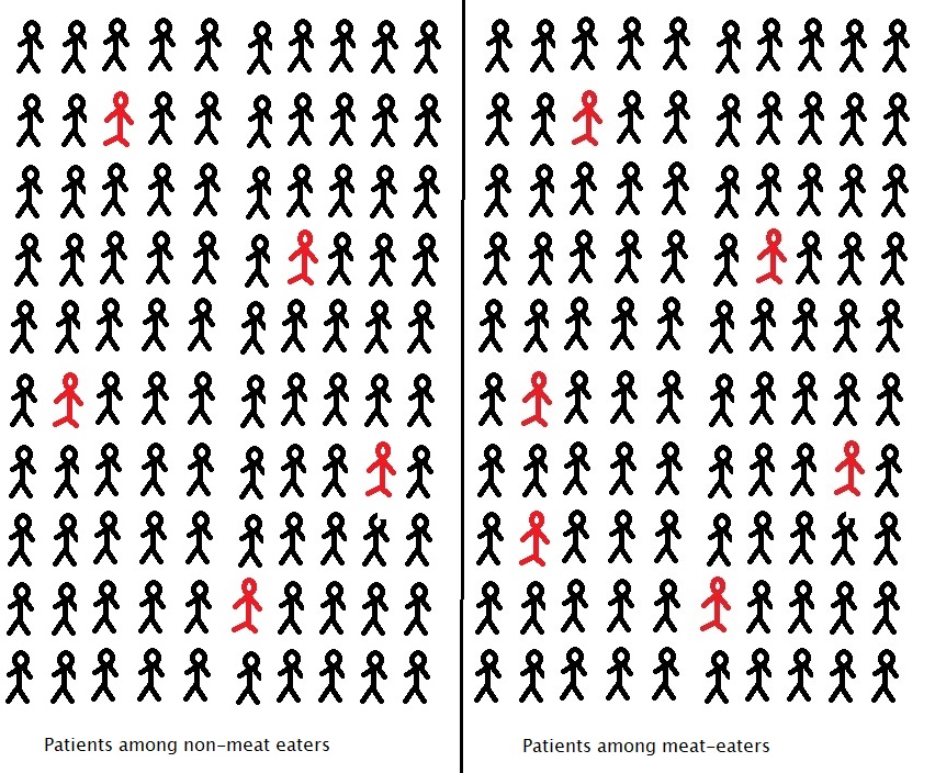
So, what is the absolute risk or the proportion of patients in the population? As per the American Cancer Society, the lifetime risk of developing colorectal cancer is about 1 in 23 (4.3%) for men and 1 in 25 (4.0%) for women. For simplicity, let’s take 5%; 18% of 5% is 0.009% or about 1 in 100. The bottom line is:

5 in 100 people can get colorectal cancer in the US, and if all of them start eating 50 g of processed meat every day, the risk increases to an additional person!

This also answers the remaining doubt on the group 1 list: Not all carcinogens in the WHO list have the same risk.

IARC Report on Processed Meat

Known Carcinogens: Cancer.org

Carcinogenicity of Processed Meat: The Lancet Oncology

How common is colorectal cancer: cancer.org

Colorectal Cancer and Meat-Eaters Read More »

Game of Chickens

Two teenagers are driving towards each other on a straight road, with an apparent show of courage to prove who can stay longer before turning off. Each teen’s expectation is to stay straight for the longest time and force the other person to swerve. The winner shines as the rebel, and the loser becomes the chicken!

Assume A and B are playing, and you can imagine four possible outcomes. 1) A chickens, 2) B chickens, 3) both chickens and 4) they collide head-on (and possibly die!). What are their payoffs? Let’s write down some, based on assumed reasons why they play this game in the first place – teen energy, naivety, happiness, pride, girls (the stereotypes, you see).

Player A
Player A StaysPlayer A Chickens
Player BPlayer B StaysA =-INF; B = -INF A = -100; B = +100
Player B ChickensA = +100; B = -100A = 0; B = 0

If player A stays and player B chickens, A gets +100, mainly in happiness, pride, etc., whereas B gets -100 (in shame!). The exact opposite happens when the fortunes are reversed.

Let’s understand the chances from player A’s point of view. If Player B stays, A can either stay (-INF) or turn away (-100), turning off and giving a better payoff. If B turns away, A can stay (+100) or move off (0). Unlike the case with the prisoner’s dilemma, the choice for A is not unique.

Given all the possibilities, what is an optimum strategy for both players? Both are courageous and stubborn. Assume player A knows B and also knows player B knows player A. It means they both try for maximum returns, but continuing the status quo will be fatal. So, there must be an exit strategy each of them must hold– to swerve away from the other, but at the last possible moment. 

In my opinion, the best option that minimises the shame and, at the same time, prevents death is when both players turn off a second before the crash!

Game of Chickens Read More »

Predict the Number – Thaler Experiment

In 1997, American behavioural economist Richard Thaler asked the readers of the Financial Times to submit a number between 0 and 100 so that the person whose number was the closest to 2/3 of the average of all numbers would be the winner. What will be your answer to this question as a rational decision-maker?

Your first step is to eliminate the obvious. The highest possible average from 0 to 100 is 100. It happens when everybody submits the number 100. It would mean the answer to the problem is (2/3) of 100 = 67. So, any number above 67 as a submission is not a rational choice.

You can’t stop there. Once you find that the rational choice for the highest number was 67, this number becomes the new highest average, and the (2/3) is 45! This iterative reasoning continues until you reach zero!

What could be an intuitive answer to this problem? Here, you assume people can randomly guess between 0 and 100, and the average is 50. (2/3) of 50 is 33. If you stop after stage 1, you submit 33 as the answer. If you continue for another round, based on the understanding that the average choice of the crowd is 33, the winner choice is 22. The number becomes 15 in the next stage and ends with 0.

So, the rational answer is 0. However, the average obtained in the actual experiment in Financial Times turned out to be 18; therefore, the winner was the one who submitted 12. The leading choices of the readers were 1, 22 and 33! When he repeated the game later, the average was 17.3, and the leaders were 1, 0 and 22.

Thaler Experiment: Financial Times

Predict the Number – Thaler Experiment Read More »

Rational Thinking and Prisoner’s dilemma

The prisoner’s dilemma is a much-discussed subject in game theory. Police arrested two individuals for their involvement in some criminal activities and put them in prison. They have adequate evidence to frame charges and hand them two years of imprisonment but not for a maximum of ten years.

Police approach a prisoner and make an offer in return to testify against the other person. If she betrays the other and the other person remains silent, she can go free. If she keeps quiet and the other person gives evidence against her, she gets the maximum punishment of 10 years. If they both remain silent, the existing term of two years continues. If they both testify against each other, they both get five years.

Imagine A is a rational decision-maker, and she assumes that a similar offer may also have gone to prisoner B. She starts from the point of view of the other person before deciding on her own. Person B has two options: remain silent or betray person A. If B remains silent, A can remain silent (2 years) or cross B (0 years). Betray B is currently the better of the two. If B testifies, A can remain silent (10 years) or betray B (5 years). Betray B is the better one here again. In other words, A has no option but to give evidence against B.

Cooperation vs Competition

Decision-making such as this starts with knowing the potential strategies of the other. Once sorted out, the player will opt for the option that protects her, irrespective of the other’s choice. 

A rational decision may not be the decision that gives the maximum payoff. In the present story, cooperation might appear as that option, where each serves two years in jail. But it was not a cooperative game, where both the parties trust each other and form a joint strategy – to remain silent. Therefore, it is not the optimal option in cases where the players compete against each other.

Cold War and Nuclear Build-Up

The Nuclear build-up between the USSR and the USA during the Cold War period is an example of a prisoner’s dilemma in real life. From the viewpoint of the USA or the USSR, the rational (strategic) option was to pile up more nuclear warheads instead of reducing them, although one has every right to argue that the latter could have been the better choice for humankind.

Rational Thinking and Prisoner’s dilemma Read More »