Poll of Polls – How FiveThirtyEight Pulls It Off

FiveThirtyEight (538) is a website based in the US that specialises in opinion poll analysis. They lead the art of election prediction, especially the US presidential, through poll aggregation strategy.

Let us look at a poll aggregator methodology and how it forecasts better than individual pollsters. Take the 2012 US presidential election, in which Obama won against Mitt Romney by a margin of 3.9%. We approach it through a simplistic model and not necessarily what 538 might have done.

Assume Top-Rated Pollsters Got It Right

Let’s try and build 12 poll outcomes that came in the last week before the election. The sample sizes of each of these polls are 1298, 533, 1342, 897, 774, 254, 812, 324, 1291, 1056, 2172 and 516 – a total of 11269 (remember that number). We don’t know anything about the details of voter preference, but we assume all the posters got it right – the 3.9% margin.

Since we don’t have any details, we simulate the survey, starting with the first pollster, 1298 samples. The following R code gives preference to 1298 people with an overall 4% advantage for Obama over Romney.

sample(c(0,1), size = 1298, replace = TRUE, prob = c(0.48, 0.52))

The code mimics choosing 1298 items from an urn containing a large number of balls having two colours, one being more prevalent than the other by a 4% chance.

Now, we follow the step-by-step procedure as we did before

  1. Number of samples – 1298
  2. Calculate the mean – In one realisation, I get 0.534
  3. Calculate the standard deviation and divide by the square root of the sample size. It’s 0.499/√1298 = 0.0139
  4. Take a 95% confidence interval and assume a standard normal distribution. (0.534 – 1.96 x 0.0139) and (0.534 – 1.96 x 0.0139). 0.50 and 0.56.

Repeat this for all the pollsters using their respective sample sizes but at a constant 4% margin on the win. One such realisation of all the 12 poles is presented below in the error plot.
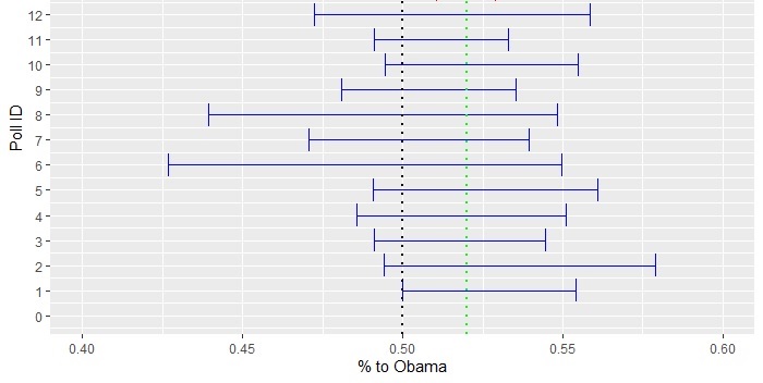
Two features of the error bars are worth noting. First, the actual outcome, 0.52, is covered by every pollster. Second, all of them covered the toss-up (a crossing over 0.5) scenario. While the first point is expected 95% of the time (by definition), the second one is more frequent for surveys with fewer participants.

Now, use the aggregator technique. Suddenly, you have 11269 samples available. Repeat all the steps above, and you get, in realisation, 0.51 and 0.53. Include that in the main plot (red error bar), and you get the following:
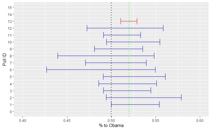
For the aggregator, the confidence interval no longer covers a toss-up.

Advantages of Aggregator Strategy 

The strength lies in the increased sampling size available to the aggregator. They also get the opportunity to select surveys that are known to be representative. For example, 538 provides a grading scheme to rate the quality of pollsters.

Five Thirty-Eight

Introduction to Data Science: Rafael Irizarry

Poll of Polls – How FiveThirtyEight Pulls It Off Read More »

When Survey Results Go Wrong

We have seen how survey methodologies based on the Central Limit Theorem work in forecasting. As you know already, CLT assumes three basic properties – independence, randomness, and the requirement to have the same underlying distribution. Together they are known as independent and identically distributed (i.i.d.).

The most common example of the system at work is election forecasting. Unlike the case with rolling dice or tossing coins, election forecasting is all about surveying the real world, and sometimes they go wrong. This time we examine some of the common reasons why the pollsters get it wrong.

Not Enough Samples

The simplest one is, of course, when there are too few numbers. You have seen that the spread of uncertainty is inversely related to the square root of the number of samples. I doubt it is a big concern; pollsters often choose sample sizes correctly, and the minimum number can be as few as 30.

Selection Bias

An example of selection bias was the calls via landlines for surveys during the US presidential polls in 2008 and 2012. Pew Research has found that the respondents of landlines, that too in the evening time when the pollsters typically make the call, were Republican-leaning. The opposite was true for cell phone users, who also happened to be the younger crowd and Obama supporters!

The second type of selection bias is also known as the house effect. Here the selection bias originates from the polling firms themselves. It happens when the polling firm has a favourite candidate and therefore publishes survey results that favour its liking.

Bradley Effect

Sometimes people simply lie, especially when their stands are at odds with socially accepted values. A classic case was in 1982 when the African-American candidate Tom Bradley, predicted to be the winner of the California governor’s race by exit polls, was lost. The respondents had clear racial preferences for the white candidate but did not want to admit that race played a role in their selection.

Selection Bias and Cell Phones

Cell Phone Users vs Landline users

House Effects of Polling Firms

Bradley Effect

Race Questions in Election

When Survey Results Go Wrong Read More »

How to Create Confidence Interval

This one is going to be one heck of a post, so hold tight. We need to start with the central limit theorem, and you know it by now. It says that the distributions of some properties of surveys, such as sum or average, follow a normal distribution if the sampling is proper. Go to this post for a refresher. By the way, don’t you think that if the sum is a distribution, the ‘average’ is also a distribution? After all, the average is the sum over a constant, the number of members in a survey.

Let me list down a few things in preparation for the upcoming roller-coaster ride.

  • Population – everything; if you go and survey everybody, you don’t need anything else, end of the story. A country’s voting is done by all its population. The outcome has no uncertainty.
  • Sample – sub-set of the population; all your statistics wizardry is required on samples. An opinion poll is on a selected sample, a few potential voters, so there is uncertainty.
  • Mean – the average of measurements. The sample mean is what we get from each survey; finding the population mean is our task.
  • Standard Deviation – a mathematical way of getting the variation of data. Use sample or population as add-ons, as before.
  • Then, there are five notations: sample size is n, the population mean is mu (μ), the population standard deviation is sigma (σ), the sample mean is Xbar (X̄), and the sample standard deviation is S.
  • Your task is to get μ and σ using one or a set of X̄ and S. All you have with you is trust in the Central Limit Theorem that says the mean of the entire distribution of all X̄ values is μ, and the standard deviation of the distribution of X̄ is σ/√n.

Mathematical Manipulations

We know that shows a normal distribution (CLT). If you subtract a constant, the outcome is still a normal distribution. So we minus μ (we don’t know μ, but that doesn’t matter). Similarly, if you divide with a constant, the distribution is still normal, so we divide with σ/√n. The new distribution is uniform, but everything else has changed now. The new mean is 0 (remember: the mean of all survey results plotted as a distribution will coincide with the population mean). And the new standard deviation is 1 (because we divided it by the exact quantity). This distribution is known by a different name – the standard normal distribution, N (of the new variable Z).

Z forms a new normal distribution with mean = 0 and standard deviation = 1. Or N(0,1)

If That Holds

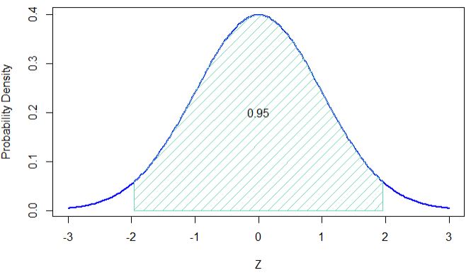
The probability that Z lies between -1.96 and +1.96 is 0.95, or 95%. If it were a normal distribution and we wanted to cover a distance of 2 times the standard deviation, shouldn’t it be plus or minus 2 and not 1.96? How did that happen? The answer is that we did not go for 2 sigma but a 95% interval. If you draw the standard normal distribution curve and check it, you will find that 95% of the distribution lies between -1.96 and +1.96.

Steps to Calculate Confidence Interval

Take the story in the previous post:

1 . Take the number of samples, n. n = 100

2. Calculate the mean of the sample, X̄. X̄ = 5

3. If you know the population standard deviation, σ. σ = 2. Divide σ with √n = 2 / √100 = 2 / 10 = 0.2. If you don’t know σ, you have to use S, the sample standard deviation. Assume S is also 2, and you get S /√n = 0.2.

4. If you know the population standard deviation, Choose the confidence interval. In our case, it was 95%. So as per the previous section, it is -(1.96 x 0.2) and +(1.96 x 0.2). That is 5 – 0.392 and 5 + 0.392 or [4.96, 5.4], which is my 95% confidence interval.

Not Over Yet

5. If you do not know the population standard deviation, As before, choose the confidence interval, which is 95%. The new interval is not between +(1.96) and -(1.96) but on a modified range. The value 1.96 becomes a function of the sample size -1 (the degrees of freedom). For smaller sample sizes, the number increases. For n = 2, it can be as large as +/- 12.71! In short, it is no longer a standard normal distribution but a t-distribution.

But we are lucky as our n is 100 (and the degrees of freedom = 99), and the multiplication factor is 1.984. -(1.984 x 0.2) and +(1.984 x 0.2). That is 5 – 0.3968 and 5 + 0.3968 or [4.96, 5.4], which is my 95% confidence interval.

T-table

Online T-distribution Calculator

How to Create Confidence Interval Read More »

Confidence Interval

Imagine you live in a town of ten thousand inhabitants. And you wanted to understand some of their habits, say, what type of food they eat, the festivals they celebrate etc. What will you do?

You go and ask every one of them. That could well be possible, as the town is not that big, 10,000 people. But you think it is a lot of effort, and you decide to employ a sampling agent. She goes to the supermarket and takes a survey of 100 people. She just did that and now tells you what she found.

She averaged the survey results and made a point estimate. She did some math and established confidence intervals to communicate. She says: “I can say with 95% confidence level that the average person of the town eats between 4.6 to 5.4 loaves of bread a day”. How do we understand her?

seagulls, thunderstorm, stormy clouds-6309501.jpg

The first thing is about the range – she gave a range [4.6 to 5.4]. It may have suggested you a mean (the bird in the picture) equals five and a spread (of its wings) of +/- 0.4. Then she says about a confidence interval as a percentage. What it means is if one does 100 such samples, 95 of the samples may have ranges that include the true average of the population – the latter is a big unknown as she never got a chance to sample everyone. This sample could be one of them, but we never know, as it was the only sample.

Some examples are below.

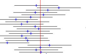
Confidence Interval of 95% of a set of 20 samples with a large range. Note that out of 20 samples, 19 of them cover the true population mean, represented as a red vertical line.
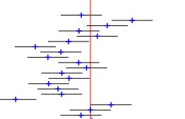
Confidence Interval of 90% of a set of 20 samples. Out of 20 samples, 18 of them cover the true population mean, represented as a red vertical line.
Confidence Interval of 50% of a set of 20 samples; about half (10) of them cover the true population mean.

Note: as the value of the confidence interval increases, the length of the wings, some multiples of the standard deviation, also increases. More on how to construct a confidence interval is in another post.

Confidence Interval Read More »

Straight Line Thinking

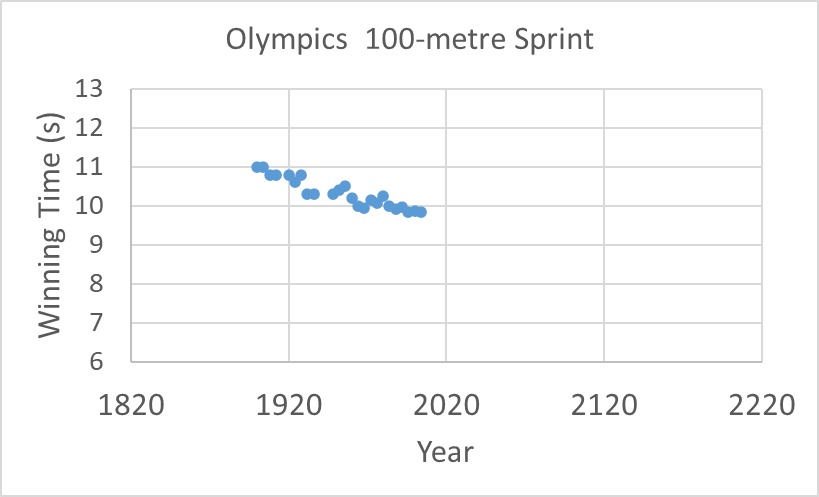
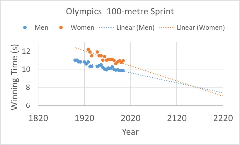
What do you see in the plot?

An ever-improving linear progression of sprint timings? Then what is your forecast, say, in the year 2200 or the year 2800?

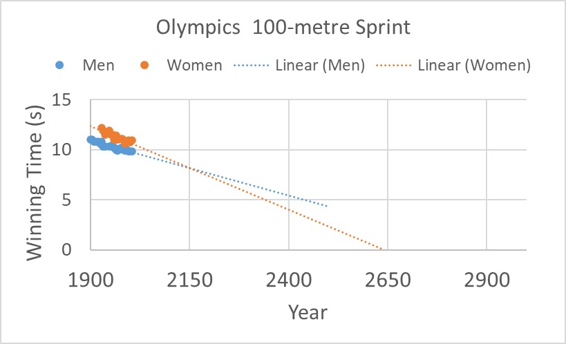
It was what happened in 2004 when a group of researchers published in the prestigious science journal nature. The article was titled, Momentous Sprint at the 2156 Olympics?: Women Sprinters are Closing the Gap on Men and May One Day Overtake Them! The study plotted men’s and women’s winning timings in Olympic 100-sprints and extrapolated to the future, similar to what I reproduced below:

And the result? A mockery of a publication in the most coveted journal in science.

The Straight Line Instinct

It is an example of what is known as the straight-line instinct, a term coined in the book Factfulness by Hans Rosling. Rosling talks about the general tendency of people to extrapolate things linearly without any regard to actual physics (or biology). Straight-line thinking is very natural to human beings. That is how we escape from a stone thrown straight at us or avoid hitting a pedestrian crossing the road ahead of us while driving.

What is Wrong with the Analysis?

First, they should have done a sanity check, especially after seeing the outcome. Some alarm bells ought to have rung not just after seeing women sprinters crossing men in the future, but more importantly at the prospect of humans crossing the 100-metre mark in zero time on extrapolating the graph even further.

Second, they did the crime of collecting a few data covering about 100 years and extrapolated over another 200. Third, they ignored the science of athletic training, early improvements and subsequent plateauing of human performance. It is like a baby in the growing phase. If you look closely, the women’s event in the Olympics started about 25 years after the men’s. So, the massive early improvements in timing lagged for many years.

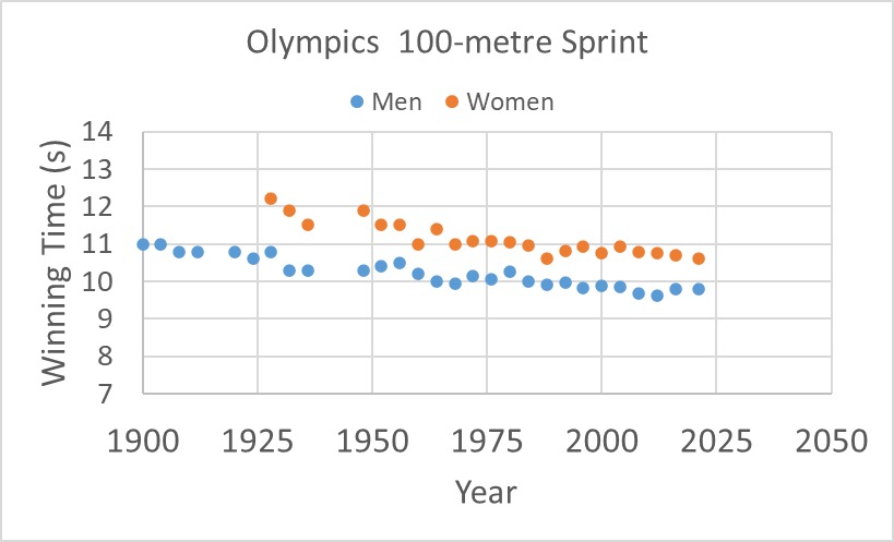
Before we close, let us have a final look at the data updated to the latest Olympics that happened in 2021.

Will they meet in future? Do you care?

Tatem et. al.: Momentous sprint at the 2156 Olympics?

Hans Rosling: Factfulness

Straight Line Thinking Read More »

The population of South Asia

Mixing is the reality of life; pure only exists in our imagination.

Humans have this love for purity and feel shame about the undeniable reality of mixing. While people in some parts of the world are proud of eating a ‘purely’ vegetarian diet, others list everything they could recollect from their harddisks to proclaim their superior ancestry. They are all right, but only for a negligibly short duration in history. Human history does not give a damn about vegetable eaters, and the same for any exclusive ancestry!

A landmark research paper came out in September 2019 in the journal Science titled, ‘The formation of human populations in South and Central Asia’. It was a report based on ancient DNA data from 523 individuals spanning the last 8000 years, from Central Asia and northernmost South Asia.

Migration of Yamnaya Steppe Pastoralists

The paper was primarily on the migration of the Eurasian Steppe to South Asia around 3000 years ago. The ‘Steppe Ancentry’ or Yamnaya culture was active around 5000 years ago in present-day Ukraine and Russia. The folks from that region had travelled to either side of the world, to Europe and South Asia. Today we talk about the guys and, perhaps some girls, who migrated to the east.

It is relevant here to talk about another DNA study published in Nature in 2009. This study genotyped 125 DNA samples of 25 different groups of India and did what is known as a Principal Component Analysis (PCA) of the data. Based on the similarities of the allele, they found a relationship between people of the North and South of India. An ancestral component, they call it ANI (Ancestral North Indian), varied from 76% for the North to 40% in the south. The remaining fraction is the ASI (Ancestral South Indians). Note that a ‘Pure’ ASI, closer to the earliest humans (travelled from Africa, of course), was not seen in that study.

Where are those people? That is next

Flashback

ASI was ‘ruling the land’ and Indus Valley Civilisation (IVC) was flourishing when the Steppe folks arrived in present-day India. But that would change soon, and the visitors would form a mix, which is the base of the continuous band from North to South that we saw earlier. So was ASI was the original one? The answer is a firm NO. ASI was a mix of what is known as AASI and a group of people with Iranian farmer ancestry. And who were this AASI? Well, they were the people who came 40,000 years ago, yes, from the cradle of homo sapiens, Africa. Of course, the Iranian farmers also went from Africa, but a few tens of thousands of years earlier.

Piecing All Together

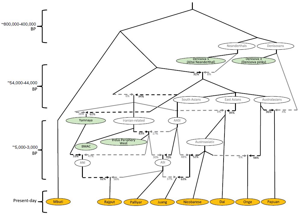
The following picture, copied from the Science paper, summarises the whole story.

Why Is It Important?

It is always fun to learn more and more about the incredible spread of homo sapiens from Africa to the rest of the world. It is equally wonderful to note how dynamic was the intermixing of population. Also, notice one irony. These results, the vivid stratification of ANI and ASI, were possible due to their obsession with endogamy in the last few hundred years. That way, they preserved the signatures of the founders or else it would have been a complete mixing of genes.

The formation of human populations in South and Central Asia: Science

Reconstructing Indian population history: Nature

The population of South Asia Read More »

Population Explosion Part 2

I want to continue the discussion on population. Again, another myth that has been dividing society for quite some time. It’s about the fertility of Muslims in India. First, check this data.

Now, you get the picture. The Muslim population has been at the receiving end of stereotyping on family sizes. As the largest minority religion, they have been looked at with a lot of suspicion by the majority in India. It was the suspicion of being overtaken one day by the minorities and, as expected, became a key discussion point in many elections.

It was a fact in the past, and it still is, that Mulsim women have an average fertility rate more than most of the other religions. It is also a fact that they made the most solid improvement in the last 20 years.

The Reality of Fertility Rates

Religious leaders advocate for more children in their community as a show of strength, and getting lost in that noise is easy. But what happens inside the family is quite different. Family size selection is often determined by economic status, coming from the need to have more ‘boys’ to support households. It has been proven beyond any doubt that female education and economic empowerment are the factors that determine family size. Check this data if you are still in doubt.

The current fertility levels of India are a powerful testimony of how communities are climbing the ladder of social and economic development. We should acknowledge this, and policymakers should strive to establish even more parity among various communities in society.

At the end of their report, Pew Research also shows a population projection for 2050.

Relax, ‘they’ have still not overtaken ‘us’!

Religious Composition of India, Pew Research

The Future of World Religions, Pew Research

National Family Health Survey, India

Census of India 2011

Population Explosion Part 2 Read More »

India’s Population Explosion

News items about population growth are sure to grab a lot of attention. For the government, it means planning, and for the public, it concerns sharing resources. For the groups with a vested interest, it is all about the ‘others’ and the potential threat they become to ‘us’. India is no exception.

That is why the news about India’s fertility rate falling below the replacement rate is very important. According to the latest National Family Health Survey 2019-21, the number of children per fertile woman in India is 2.0. In other words, from now on, the number of children born can’t match the number of parents (which is two!).

Was it a sudden phenomenon that no one knew coming? False. The fertility rate has been on a free fall since 1960—from about 5.9 to what we have today! Now, leave this post and click this Gapminder link.

Then why has the population been increasing all these years? Surely not because children were going up or the old were living longer. It is because the number of adults has been going up. To understand this, you should know the shape of India’s demography.

This population pyramid is from 2011, but an older version is not expected to be hugely dissimilar. We can do the math in another post, but remember this. Children of today (say 0 to 20 years) have to fill the large neck that appears in the pyramid. The people getting out of the system due to old age are from an even narrower side.

National Family Health Survey, India

Factfulness, Hans Rosling

Census of India 2011

India’s Population Explosion Read More »

Probabilities and Evolution

What is the probability of creating a fully developed animal or a human being? Creationists often use this argument to challenge science, but that is understandable. What is depressing is to see many scientists, too, falling into their trap.

Look at this mind-boggling probability. Think about one biological molecule in our body – haemoglobin. The molecule consists of 4 chains of amino acids, and each chain is about 146 links consisting of a possible 20 amino acids. So, to get a functional molecule, it needs to get one right out of (20)146 options. How is it then possible to have the whole human body created? Since your random processes can’t explain such ‘beautiful crafts’ of nature, you better accept my design theory!

It is a valid question, except that today’s complex systems are not formed like this. The answer lies in evolution. You and I are today because of the accumulated small changes. Not from any single change. Getting a small change is relatively easy, with about a few million unforced errors happening every day.

The complex systems we see today all originated from simpler systems. And those simpler ones, from even simpler ancestors. Until the stage, when the first life, some RNA-based self-replicating molecule, was formed! And how are they made? By chance in the chemistry laboratory of the earth using simple gases in the presence of heating, cooling and lightning. Stanley Lloyd Miller and Harold Clayton Urey proved that in 1953 by using methane, ammonia, water, hydrogen, and electric discharge to produce amino acids. Subsequent works of scientists synthesised the building bases of RNA from simple molecules.

In my post on SLC24A5 or the one on plant breeding, we have seen that a simple change in a random gene location can produce wonders. Think about it. There have been 3.5 billion years passed since the first life. Millions of trivial changes happened, a few of them passed through the sieves of nature, and a number of them got rejected to extinction. It is called natural selection.

Richard Dawkins: The Blind Watchmaker

Blind Watch Maker

Stanley L Miller, A production of Amino Acids Under Possible Primitive Earth Conditions, Science, 1953

Formation of nucleobases in a Miller–Urey reducing atmosphere, PNAS, 2017

Probabilities and Evolution Read More »

T&K Stories – 4. Anchoring and Its Impact on Our Decisions

This time we discuss another story from the paper of Tversky and Kahneman – about the biases originating from our inability to make adjustments from an initial value. In other words, the initial value anchors to our head.

To illustrate this bias: the following expressions were given to two groups of high-school students to estimate in 5 seconds.
to the first group: 1 x 2 x 3 x 4 x 5 x 6 x 7 x 8
to the second group: 8 x 7 x 6 x 5 x 4 x 3 x 2 x 1

The median estimate for the first group was 512, and that of the second was 2250 (the correct answer is 40320)!

Our Estimation of Success and Risks

Overestimation of benefits and underestimation of downsides are things we see every day. On the one hand, it was necessary for us, as a species, to make progress, yet it could seriously land in failure to deliver quality products in the end.

Conjunctive Events

Imagine, the success of a project depends on eight independent chances, each with 95% probability (almost a pass for each!). So overall, the project has (0.95)8 = 66% chance of success. Often people overestimate this as the number 0.95 gets them into a belief of surety of success. These are conjunctive events, where the outcome is a joint probability or conjunction with one other.

Disjunctive Events

A classic case of a disjunctive event is the estimation of risk. Each stage of your project has a tiny probability, about 5%, that can stop the business. What is the overall risk of failing? You know by now that you can’t multiply all those tiny numbers, instead estimate the chance not to lose in any step and then subtract it from 1. (1 – (0.95)8) = 33%. You don’t finish in one out of three cases. People underestimate risks because the starting point appears too small to be significant.

Tversky, A.; Kahneman, D., Science, 1974 (185), Issue 4157, 1124-1131

T&K Stories – 4. Anchoring and Its Impact on Our Decisions Read More »