Running t-Test on a Sample

We have been hearing about hypothesis testing a lot. But what is that in reality? We will resolve it systematically by working with samplings from a large – computer-generated – population.

What is hypothesis testing?

It is a tool to express something about a population from its small subset, known as a sample. If one measures the heights of 20 men in the city centre, does something with the data and makes a claim about men in the city, it qualifies as a hypothesis. Imagine if it was a cunning journalist who measured the heights (mean = 163 cm and standard deviation = 20 cm) and reported that the people in the city were seriously undersized (the national average is 170), a claim the mayor vehemently disputes.

So, we need someone to perform a hypothesis test assessing two mutually exclusive arguments about the city’s population and tell which one has support from the data. The mayor says the average is 170, and the journalist says it’s not.

The arguments

Null hypothesis: The population mean equals the national average (170 cm).
Alternate hypothesis: The population mean does not equal the national average (170 cm).

Build the population

The city has 100,000 men, and their height data is available to an alien. The average is, indeed, 170 cm. And do you know how she got that information? By running the following R code:

n_pop <- 100000
pop <- rnorm(n_pop, mean = 170, sd = 17.5)

Don’t you believe it? Here they are:

The journalist took a sample of 30 from it. So the statistician’s job is to verify if his number (sample mean of 163 cm at sample standard deviation of 20 cm) is possible from this population.

Test statistic

Calculating a suitable test statistic is the first step. A statistic is a measure that is applied to a sample, e.g., sample mean. If the same is done to a population, it is called a parameter. So population parameters and sample statistics. For the given task, we chose a t-test statistic by smartly combining the mean and standard deviation of the sample into a single term in the following fashion:

t = \frac{\bar{X} - \mu_0}{s/\sqrt{n}}

X bar is the sample mean
mu0 is the null value
s is the sample standard deviation and
n is the number of individuals in the sample

For the present case, it is:

t = \frac{163 - 170}{20/\sqrt{30}} = -1.92

Why is that useful?

To understand the purpose of the t-test statistics, we go back to the alien. It collected 10,000 samples, 30 data points at a time, from the population, and here is how it was obtained.

itr <- 10000

t_val <- replicate(itr, {
n_sam <- 30
sam <- sample(pop, n_sam, replace = FALSE)
t_stat <- (mean(sam) - 170)/(sd(sam) / sqrt(n_sam)) 
})

You can already suspect that our t-value of -1.92, obtained from an average of 163 cm, is not improbable for a population average of 170 cm. In other words, getting a sample mean of 163 is “natural” within the scatter (distribution) of heights. If you are not sure how t-values change, try substituting 162, and you get -2.2 (higher magnitude, further away from the middle).

t-distribution

Luckily, there has been a standard distribution that resembles the above histogram created from the subsamples. As per wiki, the t-distribution was first derived in 1876 by Helmert and Lüroth. It is of the following form. 

f(t) = \frac{\Gamma(\frac{df + 1}{2})}{\sqrt{df\pi} \Gamma(\frac{df }{2})} (1 + \frac{t^2}{df})^{-\frac{(df + 1)}{2}}

The beauty of this function is that it has only one parameter, df (number of data points – 1). The plot of the function for df = 29 is below.

x_t <- seq(- 5, 5, by = 0.01)
df <- 29

y_t <- gamma((df+1)/2)(1+(x_t^2)/df)^(-(df+1)/2)/(sqrt(df*3.14)*gamma(df/2))

plot(x_t, y_t, type = "l", main = "t-distribution for df = 29", xlab = "t value", ylab = "f(t)")

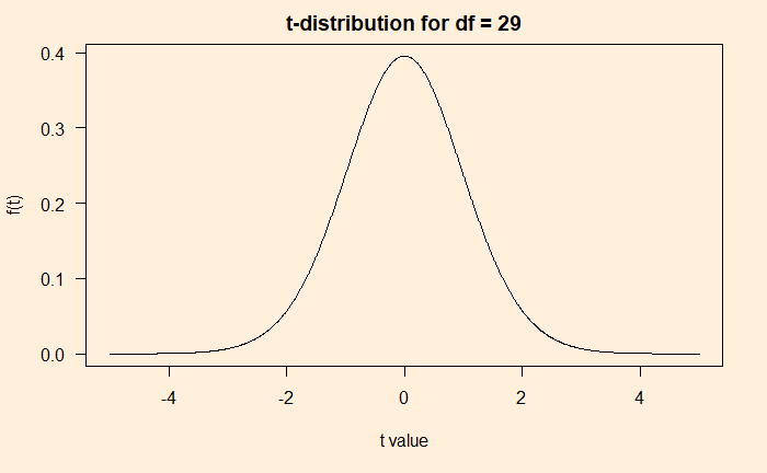
Combining distributions

Before going forward with inferences, let’s compare the sampling distribution (from 10000 samples as carried out by the alien) with the t-distribution we just evaluated.

Pretty decent fitting! Although, in reality, we never get a chance to produce the sampling distribution (the histogram), we do not need that anymore as we are convinced that the t-distribution will work instead.

Verdict of the test

The t-statistic derived from the sample, -1.92, is within the distribution if the average height of 170 cm is valid for the population. But by how much? One way to specify an outlier is by agreeing on a significance value; the statistician’s favourite is 95%. It means if the t value of the sample (the value of the x-axis) is in such a way that it is part of 95% of the distribution, then the sample mean that produced the t-value is valid. In the following figure, the 95% coverage is shaded, and our statistic is denoted as a red dot. In summary: a value of 163 cm is perfectly reasonable in the universe of 170!

Based on this, the collected data is not sufficient to dislodge the null hypothesis – a temporary respite for the mayor. Interestingly, the data can never prove he was right – it only says there is insufficient ground to reject his position.

Running t-Test on a Sample Read More »

Hypothesis Tests – What to Use

We have seen several hypothesis testing methods, such as t-tests, Z-tests, ANOVA etc. Today, we will build a flowchart to help decide what to choose. Before we select, there are a few conditions that we must satisfy.

1) We have a random sample. In case you forgot, a sample is a collection of observations. If all members are inside it, you no longer call it a sample but a population. So, the first condition says the observations must be unbiased.
2) We focus on continuous data this time.
3) The sample data should follow a normal distribution. If not, have more than 30 observations and let the central limit theorem justify you.

What is a paired sample?

Paired samples are observations on the same set of individuals, e.g. before and after or pre-intervention and post-intervention.

Hypothesis Tests – What to Use Read More »

Coin Flipping Game

Anna and Bryce are playing a game of coin flips. Anna gets one point for a head, and Bryce gets one for a tail. Whoever secures 10 points win the game. At present, Anna leads 8 – 7. What is the probability that she eventually wins?

The maximum number of games possible from now is four (a best of 19 will lead to 10, and 15 games are over). The simplest solution is to list all the possibilities that favour Anna and estimate the probabilities of those occurrences. They are

OutcomeProbability
HH 1/4
HTH 1/8
HTTH1/16
THH 1/8
TTHH1/16
THTH1/16
Total11/16 = 0.6875

Coin Flipping Game Read More »

Girl Paradox – The Simulations

You may recall the boy or girl paradox and the Bayesian explanation from the earlier two posts. Today we will perform experiments with thousands of families and count. Or simulate using the Monte Carlo method written in R. First, what is the paradox?

1) Mr X has two children. The first one is a girl, and what is the probability that both the children are girls?
2) Mr Y has two children. At least one of them is a girl, and what is the probability that both the children are girls?

Martin Gardner (1959)

We will use the replicate() function to do simulations. Before we go through the problems, let’s calculate the probability of having two girls if no other information is given.

itr <- 1000000

girl_count <- replicate(itr, {
   child <- sample(c("B","G"), size = 2, replace = TRUE, prob = c(1/2,1/2))
   child <- paste(child,collapse =" ")
    ifelse (child == "G G", "2G", "n2G") 
})

length(girl_count[girl_count == "2G"]) / length(girl_count[girl_count == "2G" | girl_count == "n2G"])

The code yields 0.25 as the answer. To explain what we did: assign “B” or “G” to two children at random using the sample() function and count the items “G G” among all the possible outcomes. Now, item 1 of the two.

itr <- 1000000

girl_count <- replicate(itr, {
    child <- sample(c("B","G"), size = 2, replace = TRUE, prob = c(1/2,1/2))
    child <- paste(child,collapse =" ")

    if(substr(child, 1, 1) == "G"){
       ifelse (child == "G G", "2G", "1G") 
    } 
})

length(girl_count[girl_count == "2G"]) / length(girl_count[girl_count == "2G" | girl_count == "1G"])

The answer is 0.5. The key difference here is that we count for two girls for only the situations where the first one is already a girl. It is achieved by searching the first member of the substring and proceeding further only if it is a “G”. Note: using the function substr() requires the library(stringr). Finally, the contentious one – item 2.

itr <- 1000000

girl_count <- replicate(itr, {
   child <- sample(c("B","G"), size = 2, replace = TRUE, prob = c(1/2,1/2))
   child <- paste(child,collapse =" ")

   if(grepl("G", child, fixed = TRUE)){
      ifelse (child == "G G", "2G", "1G") 
   } 
})

length(girl_count[girl_count == "2G"]) / length(girl_count[girl_count == "2G" | girl_count == "1G"]) 

The answer, and no surprise, is 0.33. We have used the grepl() command to find a G somewhere as the trigger to further count or not.

Tailpiece

For those who suspect my previous post about throwing dice for a double six was similar to the last one: You are right; change B and G to the sides of a die, run the simulation, and you get what you solved analytically.

itr <- 1000000

dice_count <- replicate(itr, {
  dice <- sample(c("1","2", "3", "4", "5", "6"), size = 2, replace = TRUE, prob = c(1/6, 1/6, 1/6, 1/6, 1/6, 1/6))
  dice <- paste(dice,collapse =" ")

if(grepl("6", dice, fixed = TRUE)){
  ifelse (dice == "6 6", "2-6", "1-6") 
  } 
})

length(dice_count[dice_count == "2-6"]) / length(dice_count[dice_count == "2-6" | dice_count == "1-6"])

Girl Paradox – The Simulations Read More »

It’s Raining Dice

Back to dice. Your friend casts two dice and tells you that at least one of them is a six. What is the probability that both of them are sixes?

We use Bayes’ theorem first.

P(B6|A6) = \frac{P(A6|B6)*P(B6)}{P(A6|B6)*P(B6) + P(A6|F6)*P(F6) + P(A6|S6)*P(S6) + P(A6|N6)*P(N6)}

P(B6|A6) – Probability of both six, given at least one is a six.
P(A6|B6) – Probability at least one is a six given both are six = 1
P(B6) – Prior probability for both of them is six = 1/36.
P(A6|F6) – Probability at least one is a six, given the first die is a six (and the second is not) = 1
P(F6) – Prior probability of the first die is a six (and the second is not) = (1/6)x(5/6).
P(A6|S6) – Probability at least one is a six, given the second die is a six (and the first is not) = 1
P(S6) – Prior probability of the second die is a six (and the first is not) = (1/6)x(5/6).
P(A6|N6) – Probability at least one is a six given none is size = 0
P(N6) – Prior probability of none is a six = (5/6)x(5/6).

P(B6|A6) = \frac{\frac{1}{36}}{\frac{1}{36} + \frac{5}{36} + \frac{5}{36} + 0} = \frac{1}{11}

If you are not convinced, here is a pictorial explanation:

Here are all the pairs that include at least one of them as a six. There are 11 of them in total. And there is only one that is both six. So the probability is 1 in 11.

It’s Raining Dice Read More »

Fourfold Pattern of Decision Making

In prospect theory, we have seen how human psychology slips into irrationality while understanding risks. The fourfold pattern is one such representation; of behaviours that deal with extreme probability events.

Imagine the following four cases of improving the chances of making one mln dollars.
A. 0% to 5%
B. 5% to 10%
C. 50 to 55%
D. 95 to 100%

A robot will perform the following calculations and conclude

A. (0.05 x 1,000,000 + 0.95 x 0) – 0 = $50,000
B. (0.1 x 1,000,000 + 0.90 x 0) – (0.05 x 1,000,000 + 0.95 x 0) = $50,000
C. (0.55 x 1,000,000 + 0.45 x 0) – (0.5 x 1,000,000 + 0.5 x 0) = $50,000
D. (1.0 x 1,000,000 + 0.0 x 0) – (0.95 x 1,000,000 + 0.05 x 0) = $50,000

that, all those situations lead to the same outcome – the robot has just performed an expected value calculation! But humans are not robots, and not all increment (wins or losses) has the same value.

A change from 0% to 5% is a movement from impossibility to a ray of hope. And that triggers the brain disproportionally. In other words, we overestimate that 5%. A classic example is a lottery ticket. How many of us would buy a ticket that expired a month ago? In reality, the chance of winning a lottery is almost the same as that of an expired one! This behaviour is called ‘risk-seeking‘.

On the other hand, progress from 95% to 100% is a change from possibility to certainty. An example is an out-of-court settlement. Assume you have a 95% chance of winning a lawsuit at $1 mln. Your lawyer indicated a 5% chance of losing the case and conveyed the other party’s willingness for a settlement of %750,000. Will you take it? This is ‘risk aversion‘ or underestimation of probability.

Fourfold Pattern of Decision Making Read More »

Game Theory of Marks

This one is picked from the Internet and attributed to a University of Maryland professor. The students have the opportunity to get extra marks. They can select 6 or 2 points, but with conditions: if more than 10% of the students choose 6, no one gets anything. What will be your choice?

Others pick
6 points
Your
Pick
> 10%< 10%
2 Points02
6 points06

So, in either case, you are better off or at least as good off by picking 6.

Game Theory of Marks Read More »

Sequential Lottery

Imagine there is a lottery where you pick five numbers from an urn containing 100 numbers, 1 to 100. You win the draw if you select numbers in increasing or decreasing order. For example, [23, 34, 65, 80, 94] and [69, 54, 30, 18, 9] are winning sequences, but the string [12, 43, 32, 52, 94] is not.
What is the probability of winning the lottery?

Analytical solution

Suppose you pick five numbers at random from the basket of 100. The number of ways you can arrange those five is 5! = 120. Out of those, one sequence will be in the increasing order and one in the decreasing. So the chance of getting your winning lot is (1/120) + (1/120) = 2/120 = 1.67%

Monte Carlo

itr <- 100000
lot <- replicate(itr,{
  sa <- sample(seq(1,100), 5, replace = FALSE)
  all(diff(sa) < 0) | all(diff(sa) > 0) 
})

sum(lot)*100/itr

You get an answer similar to the one before. Note that the function ‘all’ will return TRUE if all values match the criterion given a set of logical vectors. The function ‘diff’ calculates the difference between the elements ([element 2 – element 1], [element 3 – element 2] etc.) of a vector. For example,

diff(c(1,3,4,5))      # gives 2 1 1 
all(diff(c(1,3,4,5)) > 0)    # gives TRUE

Sequential Lottery Read More »

Timeless Photon

Do you know how long it takes for light from 100 lightyears away from earth to reach us? The answer is: it depends; on where you place the clock. If it is your watch, it will take 100 years. But what if the timepiece was on the photon?

As per the ‘special theory of relativity‘, the faster an object moves, the slower the time ticks for it relative to the observer.

t = t_{photon} \frac{1}{\sqrt(1 - \frac{v^2}{c^2})}

t = time as measured by a stationary observer
tphoton = time as measured by the travelling object
v = speed of the travelling object and
c = speed of light.

Now, substitute v = c; photon (light) travels with the speed of light! tphoton becomes zero.

In other words, light – from wherever it is – reaches you the moment it is born. But you may take one hundred years to catch it!

Timeless Photon Read More »

Probability of New Boy

Let’s visit our favourite subject, but after a long gap – the probability and Bayes’ theorem. Here is the question:

A new child arrives in a child-care facility that has three boys and the remaining girls. A statistician visits the centre and randomly picks up a boy child. What is the chance that the newly admitted child is a boy?

Before solving the puzzle, let the number of girls already in the centre be g. Therefore, the total number of children available for the statistician to count is 3 + 1 + g = 4 + g.

The Bayes’ equation is

P(B_n | B_r) = \frac{P(B_r | B_n) * P(B_n)}{P(B_r | B_n) * P(B_n) + P(B_r | G_n) * P(G_n)}

The terms are
P(B_n | B_r) = probability of the new child being a boy given the randomly picked is a boy
P(B_r | B_n) = probability of picking a random boy given the new child is a boy = 4 /(4+g)
P(B_r | G_n) = probability of picking a random boy given the new child is a girl = 3/ (4+g)
P(B_n) = prior probability for the new child to be a boy = 0.5
P(G_n) = prior probability for the new child to be a girl = 0.5

Substituting the terms,

P(B_n | B_r) = \frac{\frac{4}{4+g}*0.5}{\frac{4}{4+g}*0.5 + \frac{3}{4+g}*0.5} = \frac{4}{7} = 57.14\%

Probability of New Boy Read More »