You know the famous game-theory subject, the battle of the sexes. In a nutshell, it’s a game between A, who likes football and B, who prefers dance. But they also value each other’s company more than they dislike each other’s interests. Here is the overall payoff matrix written on the tastes.
B
Football
Dance
A
Football
A:10, B:5
A:0, B:0
Dance
A:0, B:0
A:5, B:10
In the classical case, A and B have 100% certainty about what the other person likes. Imagine, A becomes moody a few days a month and wants to be alone on those days. So from B’s standpoint, she knows A could be in a bad mood but doesn’t know when. So she attaches a probability, p, for A’s state.
From the side of B, there is a chance p that A wants her company.
B
Football
Dance
A
Football
A:10, B:5
A:0, B:0
Dance
A:0, B:0
A:5, B:10
And a chance (1-p) A doesn’t. And here is the corresponding payoff matrix.
B
Football
Dance
A
Football
A:0, B:5
A:10, B:0
Dance
A:5, B:0
A:0, B:10
Such cases come under the category of Bayesian Nash Equilibrium. In the original Nash equilibrium case, a player does things based on what the other player will do. In the case of Bayesian, the player acts, given what she knows the other person could do.
Look at the above graphic. There are two lines terminated with either arrowheads or arrow tails. While the length of the lines in both cases is the same, the illusion created by the form of the terminals makes our brain believe that the one on the bottom is longer. This is the Muller-Lyer illusion.
The wisdom of the crowd is an idea that stems from the fact that the average estimation by a group of people is better than by individual experts. In other words, when a large group of non-experts (not biased by knowledge!) possessing diverse opinions starts predicting a quantity, their assessment tends to form a kind of bell curve – a large pack in the middle and outliers nicely distributed on either side.
In other words, the outlier of the crowd has a lower probability of estimating it accurately. Mark this line; we need it later.
Estimating the weight
Let’s go back to Francis Galton (1907) and the story of the prize-winning-ox. It was a competition in which a crowd of about 800 people participated to predict the weight of an ox after it had been slaughtered and dressed. The person whose prediction came closer would win the prize. On the event in which Galton participated, he found a nearly normal distribution of ‘votes’, and the middlemost value, the popular choice or the vox populi, was 1207 lb which was not far from the actual dressed weight of 1198 lb.
Bidding for the meat
Now, change the scenario: the winner is no longer the predictor of weight but who will pay the most. Therefore, by definition, the people in the middle of the pack, those with a better estimation of the actual value of the meat (estimated weight x market price), are not going to get the prize. The bid belongs to the person furthest outlier (to the right) of the distribution. This is the winner’s curse – the winner is the one who overvalues the object. The only time it doesn’t apply is if the winner attaches a personal value to it, such as collecting a painting.
It is interesting to see how posterior distributions are a compromise between prior knowledge and the likelihood. An extreme, funny case is a coin that is thought to be bimodal, say at 0.25 and 0.75. But when data was collected, it gave almost equal heads and tails.
First thing first: the twin paradox is not a paradox! Now, what is it?
Before we go to the twin paradox, we must know the concept of relativity of simultaneity. It is a central concept in the special theory of relativity and happens because the speed of light is constant. A famous thought experiment is when a light flashes at the centre point of a train, running at constant velocity. To the observer inside the train, the light will reach the engine and the tail simultaneously (the same distance from the light source). But for a standing observer on the platform, the light will hit the back of the train first, as it is catching up, and strike the engine last, as it is going away from the light source. And both are right. Or the distant simultaneity depends on the reference point.
Put differently, A and B are two objects. And A moves towards the static B at a constant velocity. But from A’s vantage point, it feels stationary, and B is moving towards A. Both A and B are correct.
Over the twin paradox: Anne and Becky are twins. Becky goes away in a spaceship to a distant planet and comes back. From the stay-at-home Anne’s perspective, Becky’s clock is running slow due to the special theory of relativity. So, when she comes back, Becky will be younger than Anne. But Becky, while heading back, looks at Anne and says it was Anne who was moving towards her (in her perspective), so Anne is younger. How can both be happening? So, it’s a paradox.
Interestingly, this time, we can’t say both are right. Anne is right; Becky is the younger of the two when she returns. The only time one can claim to be at rest and the rest of the world is moving is when the moving person is moving with constant velocity. Sadly, Becky cannot claim it; she changed her direction to return and created acceleration. Remember: velocity comprises speed as well as direction. On the other hand, Anne’s version is valid as she had no acceleration but was standing at constant (zero) velocity.
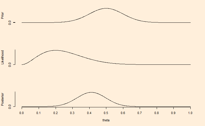
Last time, we have seen how the choice of prior impacts the Bayesian inference (the updating of knowledge utilising new data). In the illustration, a well-defined (narrower) distribution of existing understanding more or less remained the same after ten new, mostly contradicting data.
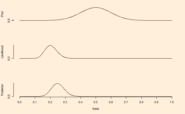
Now, the same situation but collected 100 data, with 80% leading to tails (the same proportion as before).
Now, the inference is leaning towards new compelling pieces of evidence. While Bayesian analysis never prohibits the use of broad and non-specific beliefs, the value of having well-defined facts is indisputable, as illustrated in these examples.
If there are multiple sets of prior available, it is prudent to check their impact on the posterior and map their sensitivities. Sets of priors can also be joined (pooled) together for inference.
We have seen in an earlier post how the Bayes equation is applied to parameter values and data, using the example of coin tosses. The whole process is known as the Bayesian inference. There are three steps in the process – choose a prior probability distribution of the parameter, build the likelihood model based on the collected data, multiply the two and divide by the probability of obtaining the data. We have seen several examples where the application of the equation to discrete numbers, but in most real-life inference problems, it’s applied to continuous mathematical functions.
The objective
The objective of the investigation is to find out the bias of a coin after discovering that ten tosses have resulted in eight tails and two heads. The bias of a coin is the chance of getting the observed outcome; in our case, it’s the head. Therefore, for a fair coin, the bias = 0.5.
The likelihood model
It is the mathematical expression for the likelihood function for every possible parameter. For processes such as coin flipping, Bernoulli distribution perfectly describes the likelihood function.
Gamma in the equation represents an outcome (head or tail). If the coin is tossed ‘i’ times and obtains several heads and tails, the function becomes,
The calculations
1. Uniform prior: The prior probability of the Bayes equation is also known as belief. In the first case, we do not have any certainty regarding the bias. Therefore, we assume all values for theta (the parameter) are possible as the prior belief.
The first figure demonstrates that if we have a weak knowledge of the prior, reflected in the broader spread of credibility or the parameter values, the posterior or the updated belief moves towards the gathered evidence (eight tails and two heads) within a few experiments (10 flips).
On the other hand, the prior in the second figure reflects certainty, which may have been due to previous knowledge. In such cases, contradictory data from a few flips is not adequate to move the posterior towards it.
But what happens if we collect a lot of data? We’ll see next.
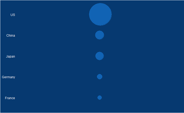
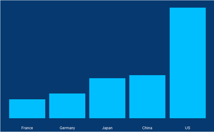
Political pitches are notorious for exaggerating facts. One example is the 2011 state of the union address of then-US President Obama. Here, he created a visual illusion using a bubble plot in the following form to represent how America’s economy compared with the rest of the top 4. Note what follows here is not the exact plot he showed but something I reproduced using those data.
Doesn’t it look fantastic? The actual values of GDP of the top 5 in 2010 were:
Country
GDP (trillion USD)
US
14.6
China
5.7
Japan
5.3
Germany
3.3
France
2.5
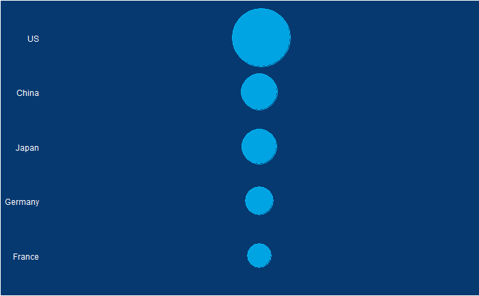
The president used bubble radii to scale the GDP numbers, which is not an elegant style of representation. It is because the area of the circle and the perspective it creates for the viewer squares with the radius. In other words, if the radius is three times, the area becomes nine times.
What would have been a better choice was to use the radius for scaling the bubble.
Or use a barplot.
Reference
The 2011 State of the Union Address: Youtube (pull up to 14:25 for the plot)
The principal-agent problem is a key concept in economic theory, which has some fascinating consequences in real life. It is easier to understand the idea using the following example.
You want to buy a house. There are a lot of potential sellers in the market; you meet one of them, agree on a price and settle the deal – a simple transaction between a buyer and a seller. But real life is more complex. You may not know where those sellers are, the market value or the paperwork that may be required to complete the process etc. So you approach a real estate agent, who has more knowledge in this topic than you, the principal. In technical language, an asymmetry of information exists.
The agent knows something that you don’t. And she realises the value (say, buy the best house at the cheapest rate) on the principal’s behalf.
A far more complex principal-agent dynamics work in a large company. A simple owner-household transaction becomes a series of relationships between the owner (shareholders) – board, board-CEO, CEO-top management, manager – technical expert etc. Here, the lower-down person (in the hierarchy) needs to act to realise the values and visions of the higher.
So what’s the problem?
The biggest one is trust. Ideally, you want the incentives of both parties (the principal and the agent) to be aligned. But since the agent has more knowledge, you suspect the former to misuse the information asymmetry to her advantage. It leads to a conflict of incentives, and the principal can’t make it if the agent did a good deal or a bad deal on your behalf.
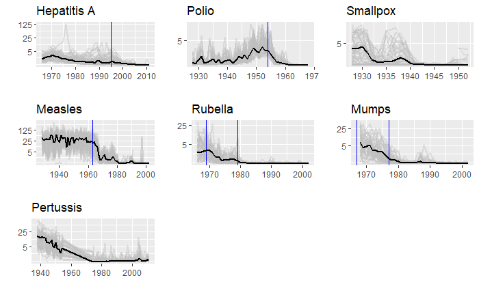
We will end this series on vaccine data with this final post. We will use the whole dataset and map how disease rates changed after introducing the corresponding vaccines. The function, ‘ggarrange’ from the library ‘ggpubr‘ helps to combine the individual plots into one.
We have used years corresponding to the introduction of vaccines or sometimes the year of licencing. In Rubella and Mumps, lines corresponding to two different years are provided to coincide with the starting point and the start of nationwide campaigns.