School, Grades and the Collider

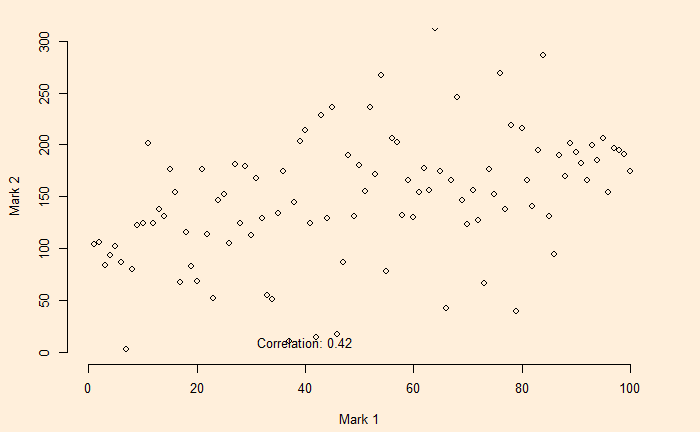
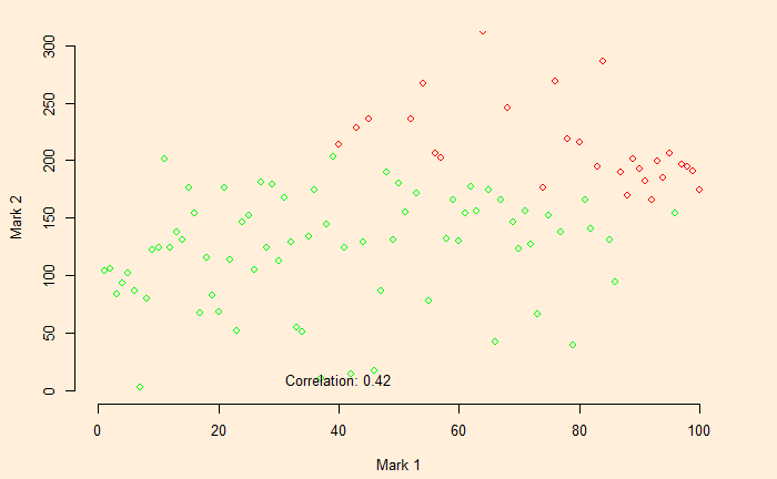
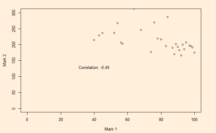
Another example of Berkson’s paradox, a collider bias, is the observed relationship, in surveys, between attending classes and grades. Here we illustrate the various possibilities and the results. Here, we explain the math using the following example.

AttendAttendDo Not
Attend
Do Not
Attend
Good
Grade
Poor
Grade
Good
Grade
Poor
Grade
300200200300

And this leads to the following conclusions:

  1. Probability of getting good grades, given the person attends classes, P(G|A) = # good grades and attend / total attend = 300/(300 + 200)= 0.6 
  2. Probability of getting poor grades, given the person attends, P(P|A) = 1 -P(G|A) = 0.4
  3. Probability of getting good grades, given the person doesn’t attend, P(G|N) = 200/(200 + 300) = 0.4
  4. Probability of getting good grades, given the person doesn’t attend, P(P|N) = 1 – P(G|N) = 0.6

Attending classes helps! But this information is never known outside. And it is where the survey gets interesting.

Imagine the survey captured the following proportions for each category.

AttendAttendDo Not
Attend
Do Not
Attend
Good
Grade
Poor
Grade
Good
Grade
Poor
Grade
0.90.50.50.1

Leading to the following Survey table.

AttendAttendDo Not
Attend
Do Not
Attend
Good
Grade
Poor
Grade
Good
Grade
Poor
Grade
27010010030

Now, calculate the probability tables, and compare with the actual.

SurveyActual
P(G|A)0.73
(270/370)
0.6
P(P|A)0.270.4
P(G|N)0.77
(100/130)
0.4
P(P|N)0.230.6

The survey tends to conclude the advantages of not attending classes!

School, Grades and the Collider Read More »

Berkson’s Paradox – Simulations

We have seen Berkson’s paradox before. It’s an erroneous correlation attributed to surveys done under specific conditions. Here we simulate a situation using R codes and illustrate the paradox.

Let’s assume a college admission process that involves two tests – test 1 and test 2. We create a set of random numbers with a positive correlation between Mark 1 and Mark 2.

x <- 1:100
y <- x + rnorm(100, 100,50)

plot(x,y, xlim = c(0,100), ylim = c(0,300),  frame.plot=FALSE, xlab = "Mark 1", ylab = "Mark 2")
text(paste("Correlation:", round(cor(x, y), 2)), x = 40, y = 10)

You will see that a reasonable positive correlation exists between the marks of the two tests (correlation coefficient = + 0.42).

Now, we impose a cut-off for the selection, i.e., the total marks (test 1 and test 2) of more than 250 to be eligible for admission.

plot(x,y, xlim = c(0,100), ylim = c(0,300),  frame.plot=FALSE,  col = ifelse(x + y > 250 ,'red','green'), xlab = "Mark 1", ylab = "Mark 2")
text(paste("Correlation:", round(cor(x, y), 2)), x = 40, y = 10)

And the eligible candidates are denoted by red circles.

Pick the red dots – the candidates who fulfilled the minimum criterion of total marks > 250 – separate and plot.

total <- data.frame(x = x, y = y, z = x+y) 
total <- total %>% filter(z > 250)

plot(total$x, total$y, xlab = "Mark 1", ylab = "Mark 2", xlim = c(0,100), ylim = c(0,300))
text(paste("Correlation:", round(cor(total$x, total$y), 2)), x = 40, y = 130)

If one surveys this college, there is a chance that the results find a negative correlation between performance in test 1 vs test 2 (in this case, a correlation of – 0.49). Imagine the first subject was science and the second was humanities! People might even attach causalities to the observations, which are biased by the selection criteria.

Berkson’s Paradox – Simulations Read More »

Skill, External Factors and Randomness

Think about it: a person attempts randomly to answer 100 multiple-choice questions – one correct answer out of four choices. What is the expected mark? Well, the first instinct could be 25. There are 100 questions, and the person who decides to attempt randomly has a one in four chance to get it right (1/4) x 100 = 25. Well, that’s an average, although, in reality, it follows a range.

Let’s run the following code to find out one such scenario.

itr <-1000

mark <- replicate(itr, {
sum(sample(c(1,0), 100, replace = TRUE, prob = c(1/4,3/4)))  
})

min(mark)
max(mark)

The output gives 12 and 40 (it will change once you repeat the calculation for randomness.

Now, we repeat the simulation with someone better at recognising the answer, i.e., a 50:50 chance of getting it right. Again, run 1000 individual runs and compare the distribution.

An extreme case is a comparison of the random with someone with 75% certainty about the answers.

Skill, External Factors and Randomness Read More »

Free Throws: What the Journalist Saw

It is a well-known fallacy to attach randomness with uniformity. And clusters are attributed to some reasoning. Here are 100 attempts on a basketball shooter who has 70% accuracy simulated.

bas_b <- sample(c(1, 0), 100, replace = TRUE, prob = c(7/10, 3/10))

You will see large clusters of successes (black dots) and a few clusters of emptiness. Overall, he is successful 70% of the time.

Imagine this happened over six games, and we show snapshots of four sub-sets of the plot as four different days of play.

Day 1 seems a very ordinary performance, followed by an excellent day 2.

Free Throws: What the Journalist Saw Read More »

Non-Ergodicity

Ergidicty is a concept in physics that equates the time average with the ensemble average of systems. In simple language, it means that the average property of a system remains the same by following one for several instances in time and averaging it (time average) or by averaging several states of the same at once (ensemble average). The first type is dynamic (changes with time), and the second is stochastic (statistical).

The assumption of ergodicity is fundamental to equilibrium statistical mechanics and, therefore, allows replacing dynamical descriptions with simpler probabilistic summaries. For example, the Brownian motion of gas molecules in a container is ergodic, meaning that a given molecule spends the same time in one half of the container as in the other half. In the coin tossing example, the average of results from tossing a fair coin infinite times equals tossing an infinite number of similar coins once.

Conversely, a stochastic process is non-ergodic when its statistics change with time. And this is what we saw in the special betting game.

Non-Ergodicity Read More »

Dunning–Kruger effect and Randomness

We have seen the Dunning-Kruger effect in the past. In his famous experiments, he collected data from 65 Cornell University graduates to verify what is known as the “above-average effect”. They made four predictions which formed the hypothesis that they wanted to test.

  1. Incompetent people overestimate their ability
  2. Incompetent individuals suffer from deficient meta-cognition abilities
  3. Incompetent people struggle with social comparison abilities
  4. Incompetent individuals can improve their insights by making them more competent

Signals and Noises

Nuhfer et al. used random number simulations to show plots of similar nature, suggesting issues with the study and the convention of using percentile plots. The graph convention holds ceiling effects wherein the lower quantile people overestimate their competency the most (more room available towards the top than the bottom). The top quantile (the competent participants) cannot overestimate by as much.

Dunning–Kruger effect and Randomness Read More »

Changepoint Analysis

This time, we will do what is known as the change point analysis using the shark attack data that we used earlier. We use R programming to evaluate the key parameters.

First, we need the “changepoint” library to be installed. We use the function, “cpt.mean” which calculates the optimal positioning and the number of changepoints for data.

cpt.mean(inv_afr$AUS)
Class 'cpt' : Changepoint Object
       ~~   : S4 class containing 12 slots with names
              cpttype date version data.set method test.stat pen.type pen.value minseglen cpts ncpts.max param.est 

Created on  : Mon Jun 26 03:47:02 2023 

summary(.)  :
----------
Created Using changepoint version 2.2.4 
Changepoint type      : Change in mean 
Method of analysis    : AMOC 
Test Statistic  : Normal 
Type of penalty       : MBIC with value, 11.35257 
Minimum Segment Length : 1 
Maximum no. of cpts   : 1 
Changepoint Locations : 24 

The program estimated the change point at 24. The next step is to plot and see what it did.

plot(cpt.mean(inv_afr$AUS))

Changepoint Analysis Read More »

Shark Attack and Randomness – A Case for Changepoint?

We have seen randomness explaining the ‘trends’ in shark attacks in South Africa. The next one is Australia. Here is the scatter from 1980-2023.

Scatter plot

It looks like two different clusters or trends, as apparent from the plot, and the change point may have happened sometime in 2000. Another way of visualising the statistical summary is to build boxplots.

Boxplot summary

A t-test is handy here to test the hypothesis (that the two trends are just by chance or not).

T-test

Aus_before <- inv_afr$AUS[which(inv_afr$Year < 2000)]
Aus_after <- inv_afr$AUS[which(inv_afr$Year > 1999)]
t.test(Aus_before, Aus_after, var.equal = TRUE)
	Two Sample t-test

data:  Aus_before and Aus_after
t = -8.6826, df = 42, p-value = 6.378e-11
alternative hypothesis: true difference in means is not equal to 0
95 percent confidence interval:
 -19.28749 -12.01251
sample estimates:
mean of x mean of y 
     5.85     21.50 

Comparison with South Africa

	Two Sample t-test

data:  SA_before and SA_after
t = 1.2881, df = 42, p-value = 0.2048
alternative hypothesis: true difference in means is not equal to 0
95 percent confidence interval:
 -0.8406907  3.8073574
sample estimates:
mean of x mean of y 
 7.900000  6.416667 

Unsurprisingly, the results show a p-value higher than the significant value (e.g., 0.05).

Shark Attack and Randomness – A Case for Changepoint? Read More »

Shark Attack and Randomness

People often quote shark attacks as examples for explaining randomness. For one, they have been sporadic. For example, here are statistics from South Africa.

Global Shark Attack – Worldmarising the Statistics.

The plot looks decent except for one outlier – 19 – in 1998.

One way to understand the pattern is to run a simulation assuming randomness and then compare the outcomes. Poisson distribution is best suited to make the check. Here is what we can do.

First, we plot the distribution of the actual data (in blue), followed by a comparison with the Poisson (in red).

Except for the outlier, the two plots are reasonably in agreement. Then, what about the shark attacks in Australia? That comes next.

Shark Attack and Randomness Read More »

Dice Polynomial

We have seen craps and how it is played based on the sum of two dice. And here is how the totals distribute. The question is: is there another way of throwing two dice (with another set of numbers on it) and playing the game of craps using the same rules.

Before finding the answer, let’s check how to represent a die. You can describe a die with this polynomial.

f(x) = x6 + x5 + x4 + x3 + x2 + x1

Rolling a pair of dice is nothing but multiplying this function with itself.

f(x) x f(x)= (x6 + x5 + x4 + x3 + x2 + x1) (x6 + x5 + x4 + x3 + x2 + x1)

x12 + 2x11 + 3x10 + 4x9 + 5x8 + 6x7 + 5x6 + 4x5 + 3x4 + 2x3 + x2

Check the table again; you will see from the coefficients and the exponents of the resulting polynomial that there is one way to roll a 12, two ways for 11 etc.

Dice Polynomial Read More »