Confusion of the Inverse

What is the safest place to be if you drive a car, closer to home or far away?

Take this statistic: 77.1 per cent of accidents happen 10 miles from drivers’ homes. You can do a Google search on this topic and read several reasons for this observation, ranging from overconfidence to distraction. So, you conclude that driving closer to home is dangerous. 

However, the above statistics are useless if you seek a safe place to drive. Because what you wanted was the probability of an accident, given that you are near or far from home, say P(accident|closer to home). And what you got instead was the probability that you are closer to home, given you have an accident P(closer to home|accident). Look at the two following scenarios. Note that P(closer to home|accident) = 77% in both cases.

Scenario 1: More drive closer to home

Home Away
Accident7723100
No
Accident
10002001200

Here, out of the 1300 people, 1077 drive closer to home.
P(accident|closer to home) = 77/1077 =0.07
P(accident|far from home) = 23/223 = 0.10
Home is safer. 

Scenario 2: More drive far from home

Home Away
Accident7723100
No
Accident
10005001500

Here, out of the 1600 people, 1077 drive closer to home.
P(accident|closer to home) = 77/1077 =0.07
P(accident|far from home) = 23/523 = 0.04
Home is worse 

This is known as the confusion of the inverse, which is a common misinterpretation of conditional probability. The statistics only selected the people who had been in accidents. Not convinced? What will you conclude from the following? Of the few tens of millions of people who died in motor accidents in the last 50 years, only 19 people died during space travel. Does it make space safer to travel than on earth? 

Confusion of the Inverse Read More »
Annie’s Table Game – The End Game

In the last exercise, we found that the frequentist solution heavily underpredicted Becky’s chances of winning the table game. This time, we will see how much that depended on the sample size. So, they continued the game but played 80 matches in total—Annie winning 50 to Becky’s 30. What are Becky’s chances of winning the next three games?

Frequentist solution 

This is not different from the previous: Based on the results, with 30 wins in 80 matches, Beck’s probability of winning a game is (3/8). That means the probability of Becky winning the next three games is (3/8)3 = 0.053.

Bayesian solution 

Run the R program we developed last time:

library(DescTools)
x <- seq(0,1,0.01)
AUC(x, choose(80,30)*x^33*(1-x)^50, from = min(x, na.rm = TRUE), to = max(x, na.rm = TRUE))  /
AUC(x, choose(80,30)*x^30*(1-x)^50, from = min(x, na.rm = TRUE), to = max(x, na.rm = TRUE)) 
0.057

And the Simulations

itr <- 1000000
beck_win <- replicate(itr, {
  beck_pro <- runif(1)
  p_5_3 <- dbinom(30, 80, beck_pro)

  if(runif(1) < p_5_3){
    game_5_3 <- 1
  }else{
    game_5_3 <- 0
  }
  
  
  if(game_5_3 == 1){
     beck_3_0 <- beck_pro^3
  } else{
     beck_3_0 <- 0
  }
  
  
  if(beck_3_0 == 0){
    win_beck <- "no"
  }else if(runif(1) < beck_3_0){
    win_beck <- "Becky"
  }else{
    win_beck <- "Annie"
  }
  
  })

sum(beck_win == "Becky")/(sum(beck_win == "Becky") + sum(beck_win == "Annie"))
0.058

Well, when the number of data points is large, the frequentist solution reaches what was simulated.

Annie’s Table Game – The End Game Read More »

Annie’s Table Game – Frequentist vs Bayesian 

See the story and numerical experiments in the previous post. Annie is currently leading 5-3; what is the probability that Becky will reach six and win the game?

Frequentist solution 

Based on the results so far, 3 wins in 8 matches, Beck’s probability of winning is (3/8). That means the probability of Becky winning the next three games (to reach 6 before Annie wins another, which will make her 6) is (3/8)3 = 0.053.

Bayesian solution 

First, we write down the Bayes equation. The probability of B winning the game, given A is leading 5-3, 

\\ P(B|A_{5-3}) = \frac{P(A_{5-3}|B)*P(B)}{P(A_{5-3})}

Let’s start with the denominator. If p represents the probability of Becky winning a game, the probability of a 3-5 or 3 in 8 result is obtained by applying the binomial equation. The denominator is the sum of all possible scenarios (p values from 0 to 1). In other words, The denominator is,

\\ P(A_{5-3}) = \int_0^1 _8C_3 p^3 (1-p)^5

We use an R shortcut to evaluate the integral as the area under the curve using the ‘AUC’ function from the ‘DescTools’ library.

library(DescTools)
x <- seq(0,1,0.01)
AUC(x, choose(8,3)*x^3*(1-x)^5, from = min(x, na.rm = TRUE), to = max(x, na.rm = TRUE)) 
0.1111

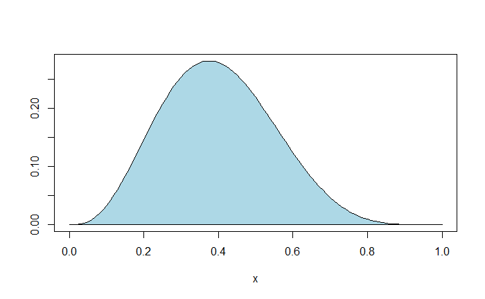
And here is the area. 

plot(x, choose(8,3)*x^3*(1-x)^5, type="l", col="blue", ylab = "")
polygon(x, choose(8,3)*x^3*(1-x)^5, col = "lightblue")

The numerator is the multiplication of the likelihood function with the prior probability of Becky winning three games. We will use a binomial equation as the prior function and p x p x p = p3 as P(B). 

\\ P(A_{5-3}|B)*P(B) = 8C_3 p^3 (1-p)^5 p^3 \\ \\ 8C_3 p^6 (1-p)^5

Again, the area under the curve all possible p values (0 -1),

AUC(x, choose(8,3)*x^6*(1-x)^5, from = min(x, na.rm = TRUE), to = max(x, na.rm = TRUE)) 
0.0101

The required Bayesian posterior is 0.0101/0.1111 = 0.0909

To sum up

The Bayesian estimate is almost double compared to the frequentist. The Bayesian estimate is much closer to the results we saw earlier. Does this make Bayesian the true winner? We’ll see next. 

Annie’s Table Game – Frequentist vs Bayesian  Read More »

Annie’s Table Game

Annie and Becky are playing a game in which the aim is to secure six points first. The Casino randomly rolls a ball onto the table, and the point at which the ball rests is marked. The Casino then rolls another ball at random. If it comes to rest to the left of the initial mark, Annie wins the point; to the right, Becky wins. If Annie is currently leading 5-3, what is the probability that Becky will win the game?

Before we get into statistical methods, we will play the game a million times using R. 

First step: Becky’s chance of winning any game is a random number with uniform probability. If that is the case, the probability of Annie leading 5-3 (or Becky winning 3 out of 8 games) is given by binomial distribution.

beck_pro <- runif(1)
p_5_3 <- dbinom(3, 8, beck_pro)

That gives the probability of having a 5-3 lead for Annie, but that doesn’t mean it will happen for sure. For that to happen, the estimated probability must be greater than a random number between 0 and 1.

  if(runif(1) < p_5_3){
    game_5_3 <- 1
  }else{
    game_5_3 <- 0
  }

Thus, we established instances where Annie was leading 5-3. We will estimate the probability of Becky winning the next three games. 

  if(game_5_3 == 1){
     beck_3_0 <- beck_pro^3
  } else{
     beck_3_0 <- 0
  }

Like we did before, a random number is generated, and if it is less than the probability of Becky winning the next three games, Becky wins; otherwise, Annie wins. 

 if(beck_3_0 == 0){
    win_beck <- "no"
  }else if(runif(1) < beck_3_0){
    win_beck <- "Becky"
  }else{
    win_beck <- "Annie"
  }
  
  })

Calculate this a million times and estimate the proportion of Becky’s win over total wins.

itr <- 1000000
beck_win <- replicate(itr, {
  beck_pro <- runif(1)
  p_5_3 <- dbinom(3, 8, beck_pro)

  if(runif(1) < p_5_3){
    game_5_3 <- 1
  }else{
    game_5_3 <- 0
  }
  
  
  if(game_5_3 == 1){
     beck_3_0 <- beck_pro^3
  } else{
     beck_3_0 <- 0
  }
  
  
  if(beck_3_0 == 0){
    win_beck <- "no"
  }else if(runif(1) < beck_3_0){
    win_beck <- "Becky"
  }else{
    win_beck <- "Annie"
  }
  
  })

sum(beck_win == "Becky")/(sum(beck_win == "Becky") + sum(beck_win == "Annie"))
0.09057296

Introduction to Bayesian Statistics – A Beginner’s Guide: Woody Lewenstein

What is Bayesian statistics?: Nature Biotechnology,  volume 22, 177–1178 (2004)

Annie’s Table Game Read More »

The Bayesian Runner

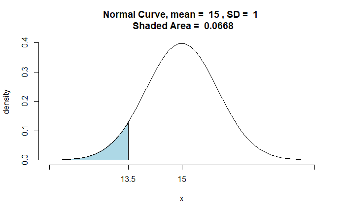
Becky loves running 100-meter races. The run timing for girls her age follows a normal distribution with a mean of 15 seconds and a standard deviation of 1s. The cut-off time to get into the school team is 13.5 seconds. If Becky is on the school running team in 100 meters, what is the probability that she runs below 13 seconds?

Without any other information, we can use the given probability distribution to determine the chance of Becky running under 13 seconds.

pnormGC(13,region="below", mean=15,sd=1.,  graph=TRUE) 

Since we know she is in the school team, we can update the probability as per Bayes’ theorem. Let’s use the general formula of Bayes’ theorem here:

\\ P(13|T) = \frac{P(T|13)*P(13)}{P(T)}

The first term in the numerator, P(T|13) = 1 (the probability of someone in the team with a cut-off of 13.5 s, given her timing is less than 13s). We already know the second term, P(13), 0.0228.

The denominator, P(T), is the probability of getting on the team, which is nothing but the chance of running under 13.5 seconds. That is, 

pnormGC(13.5,region="below", mean=15,sd=1.,graph=TRUE)

Substituting P(T) = 0.0668 in the Bayes equation,

P(13|T) = 0.0228/0.0668 = 0.34 or 34%

The Bayesian Runner Read More »

Begging the Question

A person new to religion may have questions about the credibility of its belief system. For example, how do I know the way God operates? A person with a Christian belief system will tell you it’s written in the Bible. But how do I know the Bible is telling the truth? I did a search, and one of the results on the validity of the scriptures was the King James Bible online. The first one was:

2 Timothy 3:16 – All scripture is given by inspiration of God, and is profitable for doctrine, for reproof, for correction, for instruction in righteousness:” 

If you are happy with the answer, like millions of people, you have committed the fallacy of begging the question. Begging the question is a complicated way of describing a circular reasoning, where an argument’s premise assumes the truth of the conclusion.

An argument has three parts:
1. Claim or conclusion – presented upfront
2. Support or evidence – presented to back the claims
3. Warrant or major premise – hidden in the argument but bridges the support to the claim.

Consider the following argument. 

In the fallacy of circular argument, the claim (Bible is telling the truth) takes the evidence (verses from the book of Timothy) from the same book to prove the claim.

Data & Statistics on Autism Spectrum Disorder: CDC

Begging the Question Read More »

Liar Puzzle

Annie says Becky is lying
Becky says Carol is lying
Carol says both Annie and Becky are lying

Who is lying, and who is telling the truth?

  1. If Carol is telling the truth, then Annie (and Becky) is lying. In that case, Becky is not lying (opposite of what Annie, the ‘liar’ said). This is a contradiction. Therefore, Carol is lying.
  2. Since Carol is lying, the person who identified that correctly, Becky, must be telling the truth
  3. If Becky is telling the truth, the first statement is incorrect. Therefore, the person who made the first statement, Annie, is also lying.

Liar Puzzle Read More »

Implied Probabilities and Fractional Odds

If ‘moneyline’ is the term used in American betting, it’s ‘fractional odds’ for the UK. So, for today’s premier league match between Chelsea and Everton, the following are the odds.

HomeDrawAway
14/1910/319/5

This means that if you bet on home, i.e., Chelsea (the match is played in Chelsea’s backyard) and win, you get a profit of £14 for every £19 placed. In other words, you bet £19 and get back £14+£19 = £33.

As before, let’s estimate the implied probability based on the (fair) expected value assumption.
E.V = p x 14 – (1-p) x 19 = 0
14p + 19p – 19 = 0
p = 19/(14 + 19) = 0.576 = 57.6%

As a shortcut: for 14/19, p = 1/[(14+19)/19].

And for the next two
Draw: p (10/3) = 1/[(10+3)/3] = 0.231 = 23.1%
Away (Everton win): p (19/5) = 1/[(19+5)/5] = 0.208 = 20.8%

As expected, the sum of probabilities is not 100% but 101.5%; the house must win.

Implied Probabilities and Fractional Odds Read More »

Implied Probabilities vs Moneyline

We have seen how to interpret the betting odds or moneyline. Take, for example, the NBA odds for one of tonight’s matches.

TeamMoneyline
Washington Wizards+340
Boston Celtics-450

If you place $100 on the Wizards, and they win, you get $440, suggesting a profit of $340 upon winning (and you lose $100 if they lose).
On the other hand, if you bet $450 on the Celtics, and they win, you get $550 (and a loss of $450 if they lose). Your profit for winning is $100.

Implied probability

Let’s apply the expected value concept to this problem. Let p be the probability of winning the prize upon betting on the Wizards. For this to be a fair gamble,
the expected value = p x 340 – (1-p) x 100 = 0
p = 100/440 = 0.227 or 22.7%; this is an implied probability of the bet.

Let q be the probability for the Celtics.
the expected value = q x 100 – (1-q) x 450 = 0
q = 450/550 = 0.818 or 81.8%

Suppose you add the two probabilities, p + q = 104.5%. It is more than 100%, suggesting they are not the actual probabilities (fair odds) of winning the (NBA) game. Since the actual win probabilities of teams must add up to 100%, the sum p + q must be lower than that obtained in the expected value calculations. Therefore, at least one of the expected values must be < 0.

104.5% may be understood as putting $104.5 the money at risk to get $100 back. The difference (104.5 – 100)/104.5 is the bookie’s edge built into the bet.

Implied Probabilities vs Moneyline Read More »

Employee Attrition Dataset

We continue using the ‘tigerstats’ package to analyse the ‘IBM HR Analytics Employee Attrition & Performance’ dataset, a fictional data set created by IBM data scientists and taken from Kaggle. The dataset contains various parameters related to attribution,

Em_data <- read.csv("D:/04Compute/Web/Employee-Attrition.csv")
str(Em_data)
'data.frame':	1470 obs. of  35 variables:
 $ Age                     : int  41 49 37 33 27 32 59 30 38 36 ...
 $ Attrition               : chr  "Yes" "No" "Yes" "No" ...
 $ BusinessTravel          : chr  "Travel_Rarely" "Travel_Frequently" "Travel_Rarely" "Travel_Frequently" ...
 $ DailyRate               : int  1102 279 1373 1392 591 1005 1324 1358 216 1299 ...
 $ Department              : chr  "Sales" "Research & Development" "Research & Development" "Research & Development" ...
 $ DistanceFromHome        : int  1 8 2 3 2 2 3 24 23 27 ...
 $ Education               : int  2 1 2 4 1 2 3 1 3 3 ...
 $ EducationField          : chr  "Life Sciences" "Life Sciences" "Other" "Life Sciences" ...
 $ EmployeeCount           : int  1 1 1 1 1 1 1 1 1 1 ...
 $ EmployeeNumber          : int  1 2 4 5 7 8 10 11 12 13 ...
 $ EnvironmentSatisfaction : int  2 3 4 4 1 4 3 4 4 3 ...
 $ Gender                  : chr  "Female" "Male" "Male" "Female" ...
 $ HourlyRate              : int  94 61 92 56 40 79 81 67 44 94 ...
 $ JobInvolvement          : int  3 2 2 3 3 3 4 3 2 3 ...
 $ JobLevel                : int  2 2 1 1 1 1 1 1 3 2 ...
 $ JobRole                 : chr  "Sales Executive" "Research Scientist" "Laboratory Technician" "Research Scientist" ...
 $ JobSatisfaction         : int  4 2 3 3 2 4 1 3 3 3 ...
 $ MaritalStatus           : chr  "Single" "Married" "Single" "Married" ...
 $ MonthlyIncome           : int  5993 5130 2090 2909 3468 3068 2670 2693 9526 5237 ...
 $ MonthlyRate             : int  19479 24907 2396 23159 16632 11864 9964 13335 8787 16577 ...
 $ NumCompaniesWorked      : int  8 1 6 1 9 0 4 1 0 6 ...
 $ Over18                  : chr  "Y" "Y" "Y" "Y" ...
 $ OverTime                : chr  "Yes" "No" "Yes" "Yes" ...
 $ PercentSalaryHike       : int  11 23 15 11 12 13 20 22 21 13 ...
 $ PerformanceRating       : int  3 4 3 3 3 3 4 4 4 3 ...
 $ RelationshipSatisfaction: int  1 4 2 3 4 3 1 2 2 2 ...
 $ StandardHours           : int  80 80 80 80 80 80 80 80 80 80 ...
 $ StockOptionLevel        : int  0 1 0 0 1 0 3 1 0 2 ...
 $ TotalWorkingYears       : int  8 10 7 8 6 8 12 1 10 17 ...
 $ TrainingTimesLastYear   : int  0 3 3 3 3 2 3 2 2 3 ...
 $ WorkLifeBalance         : int  1 3 3 3 3 2 2 3 3 2 ...
 $ YearsAtCompany          : int  6 10 0 8 2 7 1 1 9 7 ...
 $ YearsInCurrentRole      : int  4 7 0 7 2 7 0 0 7 7 ...
 $ YearsSinceLastPromotion : int  0 1 0 3 2 3 0 0 1 7 ...
 $ YearsWithCurrManager    : int  5 7 0 0 2 6 0 0 8 7 ...

barchartGC

barchartGC(~Gender,data=Em_data)
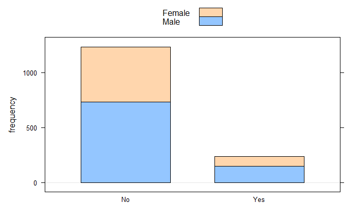
barchartGC(~Attrition+Gender,data=Em_data, stack = TRUE)

xtabs

xtabs(~Attrition+MaritalStatus,data=Em_data)
         MaritalStatus
Attrition Divorced Married Single
      No       294     589    350
      Yes       33      84    120
xtabs(~Attrition+Gender,data=Em_data)
         Gender
Attrition Female Male
      No     501  732
      Yes     87  150

CIMean

CIMean(~MonthlyIncome,data=Em_data)

ttestGC

ttestGC(~MonthlyIncome,data=Em_data)
Inferential Procedures for One Mean mu:

Descriptive Results:

variable       mean     sd       n          
MonthlyIncome  6502.931 4707.957 1470       

Inferential Results:

Estimate of mu:	 6503 
SE(x.bar):	 122.8 

95% Confidence Interval for mu:

          lower.bound         upper.bound          
          6262.062872         6743.799713      
ttestGC(~Age,data=Em_data)
Inferential Procedures for One Mean mu:

Descriptive Results:

variable  mean     sd       n          
Age       36.924   9.135    1470       

Inferential Results:

Estimate of mu:	 36.92 
SE(x.bar):	 0.2383 

95% Confidence Interval for mu:

          lower.bound         upper.bound          
          36.456426           37.391193 

Employee Attrition Dataset Read More »