November 2023

Bayes Factor and p-Value Threshold

Blind faith in p-value at 5% significance (p = 0.05) has contributed to a lack of credibility in the scientific community. It has affected the class, ‘discoveries’ more than anything else. Although the choice of threshold p-value = 0.05 was arbitrary, it has become a benchmark for studies in several fields.

It is easier to appreciate the issue once you understand the Bayes factor concept. We have established the relationship between the prior and posterior odds (of discovery) in an earlier post:
Posterior Odds = BF10 x Prior Odds

Studies show that the prior odds of typical psychological studies are 1:10 (H1 relative to H0). For clarity, H1 represents the hypothesis leading to a finding, and H0 is the null hypothesis. In such a context, a p-value, which is equivalent to a Bayes factor of ca. 3.4, makes the following transformation.

Posterior Odds = 3.4 x (1/10) = 0.34 ~ (1/3); the odds are still in favour of the null hypothesis.

On the other hand, if the threshold p is 0.005 (equivalent to a BF = 26),
Posterior Odds = 26 x (1/10) = 2.6 (2.6/1); more in favour of the discovery.

Reference

Redefine statistical significance: Nature human behaviour

Bayes Factor and p-Value Threshold Read More »
Bayes Factor and Rare Diseases

Let’s revisit Sophie and the equation of life (a.k.a. Bayes’ theorem). We know that the chance of breast cancer became about 12%, starting from a state of no symptoms and a positive test result. That too from a test that has 95% sensitivity and 90% specificity. And the secret behind this mysterious result was the low prevalence or prior probability of the disease.

P(D|TP) = P(TP|D) x P(D) /[P(TP|D) x P(D) + P(TP|!D) x P(!D)]

Here, TP represents test positive, D denotes disease and !D is no disease.

Rare disease

How do you describe a rare disease? As a simple approximation, let’s define it as an illness with a chance of 1% or lower to occur. We’ll now apply the Bayes’ rule for a few cases of P(D) (0.01, 0.005, 0.001, etc) and see how the probability updates when the test comes positive.

P(D)
Prior
P(D|TP)
Posterior
Posterior
/ Prior
(ratio)
0.010.0888.8
0.0050.0469.2
0.0010.00949.4

Can you estimate the Bayes factor for the above case?

Bayes FactorD-!D = P(TP|D) / P(TP|!D)
P(TP|D) = sensitivity = 0.95
P(TP|!D) = 1 – specificity = 1 – 0.9 = 0.1
BFD-!D = 0.95 / 0.1 = 9.5

As a heuristic, for rare diseases, the updated chance of having the disease post a positive diagnostics equals Bayes factor x prevalence.

Bayes Factor and Rare Diseases Read More »

Bayes Factor – Continued

Let’s progress further the concept of Bayes Factor (BF). In the last post, the BF was defined in favour of the null hypothesis (BF01). From now on, we focus on BF10 or the Bayes factor in favour of the alternate hypothesis.

Bayes Factor10 = P(Data|H1) / P(Data|H0)

As per Bayes theorem:
P(H1|D) = [P(D|H1) P(H1)] / P(D)
P(H0|D) = [P(D|H0) P(H0)] / P(D)
[P(H1|D) / P(H0|D)] = [P(D|H1) P(H1)] / [P(D|H0) P(H0)]
[P(H1|D) / P(H0|D)] = [P(D|H1) / [P(D|H0)] [P(H1)] / P(H0)]
Posterior Odds = BF10 x Prior Odds

This definition is significant in determining the strength of the alternate hypothesis given the experimental data or P(H1|D). Note that an experimenter is always interested in it, but the traditional hypothesis testing and p-values never helped her to know it. Let’s see how it works:

Let the prior probability for your hypothesis be 0.25 (25%), which is 1:3 prior odds (note: P(H1) + P(H0) = 1 and P(H1|D) + P(H0|D) = 1). And the BF10 is 5, which is pretty moderate evidence and is not far from a p-value of 0.05. The posterior odds become 5:3 (P(H1|D) / P(H0|D)). This corresponds to a posterior probability for the alternate hypothesis (P(H1|D)) = 5/8 = 0.625 (62.5%).

So, a Bayes Factor of 5 has improved the prior probability of the hypothesis from 25% to 62.5%.

Bayes Factor – Continued Read More »

Bayes Factor

Most of the hypothesis testing we have seen so far comes under the category of what is known as the null hypothesis significance testing (NHST). In this framework, we have two competing hypotheses:

  1. The Null Hypothesis, H0, where there is no impact of an intervention
  2. Alternate Hypothesis, HA, where there is an impact of the intervention.

Hypothesis testing aims to collect data (evidence) and assess the fit for one of the above models. At the end of NHST, you either ‘reject’ or ‘fail to reject’ your Null hypothesis – at a specified significance value – using the well-known p-value.

p-value ~ P(Data|H0)

On the contrary, we can define a ratio that gives equal weightage for the null and the alternative hypotheses. That is the Bayes Factor. It compares the probability of the data under one hypothesis with the probability under the other.

Bayes Factor01 = P(Data|H0) / P(Data|H1)

If BF01 > 1, the data is likely supporting H0
If BF01 < 1, the data is likely supporting H1

Bayes Factor Read More »

Friedman test

Let’s work out another non-parametric hypothesis test – analogous to repeated measures ANOVA, the Friedman test. The way it works is exemplified by analysing ten runners who participated in a training program. The following are the measured heart rates at regular intervals. Your task is to inspect if there is a significant difference in the heart rate of patients across the three time points.

H_Rate <-  matrix(c(150, 143, 142,
                  140, 143, 140,
                  160, 158, 165,
                  145, 140, 138,
                  138, 130, 128,
                  122, 120, 125,
                  132, 131, 128,
                  152, 155, 150,
                  145, 140, 140,
                  140, 137, 135),
                nrow = 10,
                byrow = TRUE,
                dimnames = list(1:10, c("INITIAL", "ONE WEEK", "TWO WEEKS")))
INITIAL ONE WEEK TWO WEEKS
1      150      143       142
2      140      143       140
3      160      158       165
4      145      140       138
5      138      130       128
6      122      120       125
7      132      131       128
8      152      155       150
9      145      140       140
10     140      137       135

The null hypothesis, H0: HR1 = HR2 = HR3 (mean heart rates across the intervals are all equal)
The alternative hypothesis, HA: There is a difference (at least one) during the interval.

The following command can execute the Friedman test,

friedman.test(H_Rate)
	Friedman rank sum test

data:  H_Rate
Friedman chi-squared = 5.8421, df = 2, p-value = 0.05388

The p-value is 0.053, which is greater than the significance value of 0.05; the evidence is not sufficient to reject the null hypothesis.

Friedman test Read More »

Non-Parametric ANOVA – Kruskal–Wallis test

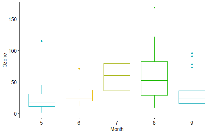
Here are five months of quality data on Ozone concentration. The task is to test if one month’s data is significantly different from any other month’s.

The first thing to graph the monthly variations of ozone in summary plots: a boxplot is one good choice.

library(ggpubr)
data("airquality")
AQ_data <- airquality
ggboxplot(AQ_data, x = "Month", y = "Ozone", 
          color = "Month", palette = c("#00AFBB", "#E7B800", "#a0AF00", "#17B800", "#20AFBB"),
        ylab = "Ozone", xlab = "Month") +
theme(legend.position="none")

Getting quantitative

Let’s do a hypothesis test. A few quick Shapiro tests suggest only month 7 followed a normal distribution. So, we will use a non-parametric test. The Kruskal–Wallis test is one of them.

kruskal.test(Ozone ~ Month, data = airquality)
	Kruskal-Wallis rank sum test

data:  Ozone by Month
Kruskal-Wallis chi-squared = 29.267, df = 4, p-value = 6.901e-06

Yes, monthly behaviours are not similar. If you want pair-wise testing, we can use a pair-wise Wilcoxon rank-sum test.

pairwise.wilcox.test(AQ_data$Ozone, AQ_data$Month)
	Pairwise comparisons using Wilcoxon rank sum test with continuity correction 

data:  AQ_data$Ozone and AQ_data$Month 

  5      6      7      8     
6 0.5775 -      -      -     
7 0.0003 0.0848 -      -     
8 0.0011 0.1295 1.0000 -     
9 0.4744 1.0000 0.0060 0.0227

P value adjustment method: holm 

The conclusion: Significant differences are seen:
Month 5 vs Month 7 and Month 8
Month 9 vs Month 7 and Month 8

Non-Parametric ANOVA – Kruskal–Wallis test Read More »

Shapiro-Wilk test – Test for Normality

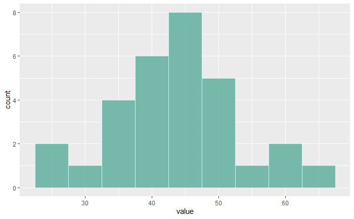
In the last post, we used a non-parametric hypothesis test, the Wilcoxon Signed Rank test. The p-value showed that the evidence was not sufficient to reject the null hypothesis. However, the histogram suggests that the data was reasonably a normal distribution.

Shapiro-Wilk test is a formal way of testing whether the data follows a normal distribution or not. The test has a null hypothesis that the sample comes from a normally distributed population. The test statistics, W has the following formula:

W = \frac{(\sum a_i x_i)^2}{\sum(x_i - \bar{x})^2}

We can apply the Shapiro-Wilk test to our data using the following R code:

diab <- c(35.5, 44.5, 39.8, 33.3, 51.4, 51.3, 30.5, 48.9, 42.1, 40.3, 46.8, 38.0, 40.1, 36.8, 39.3, 65.4, 42.6, 42.8, 59.8, 52.4, 26.2, 60.9, 45.6, 27.1, 47.3, 36.6, 55.6, 45.1, 52.2, 43.5)

shapiro.test(diab)
	Shapiro-Wilk normality test

data:  diab
W = 0.98494, p-value = 0.9361

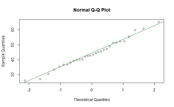
The p-value is quite high, and the null hypothesis is not rejected. The same conclusion may be obtained by doing a q-q plot as follows.

qqnorm(diab)
qqline(diab, col = "darkgreen")

Shapiro-Wilk test – Test for Normality Read More »

Wilcoxon Signed Rank Test – R Program

We will use R to perform the hypothesis test using the Wilcoxon Signed Rank Test.

The expected median age for the onset of diabetes is 45 years. The following is a list of 30 people tracking their onset of diabetes. Test whether the evidence supports the hypothesis.

diab <- c(35.5, 44.5, 39.8, 33.3, 51.4, 51.3, 30.5, 48.9, 42.1, 40.3, 46.8, 38.0, 40.1, 36.8, 39.3, 65.4, 42.6, 42.8, 59.8, 52.4, 26.2, 60.9, 45.6, 27.1, 47.3, 36.6, 55.6, 45.1, 52.2, 43.5)

The Null Hypothesis, H0: Median equals 45
The Alternate Hypothesis, H1: Median does not equal 45

wilcox.test(diab, mu = 45.0, alternative = "two.sided")
	Wilcoxon signed rank exact test

data:  diab
V = 200, p-value = 0.5158
alternative hypothesis: true location is not equal to 45

The p-value is 0.51, which is higher than 0.05 (5% significance), and therefore, the null hypothesis can not be rejected.

Since the histogram of the data appears reasonably normal, it would be interesting to test using the parametric method, such as the t-test.

t.test(diab, mu = 45.0, alternative = "two.sided")
	One Sample t-test

data:  diab
t = -0.54461, df = 29, p-value = 0.5902
alternative hypothesis: true mean is not equal to 45
95 percent confidence interval:
 40.51408 47.59925
sample estimates:
mean of x 
 44.05667 

Wilcoxon Signed Rank Test – R Program Read More »

Wilcoxon Signed Rank Test

We continue with the same dataset but use another type of non-parametric test – the Wilcoxon Signed Rank Test. Here, not only the sign of the observation counts but also the distance of departure from the median.

Case #Drug A
112.3
213.1
311.3
410.1
514.0
613.3
710.5
812.3
910.9
1011.9

The Null Hypothesis, H0: Median = 13.0
The Alternate Hypothesis, H1: Median < 13.0

Steps

  1. Estimate the difference from the null hypothesis (median = 13.0)
  2. Calculate the absolute value
  3. Estimate the rank of the list, with the smallest absolute difference getting the lowest rank
  4. Add the sign (from the difference of step 1) to the rank
  5. Add all positives and negatives separately.
  6. Take the smaller of the two and check against the table of critical values.
Drug ADifferenceAbs
Difference
RankSigned
Rank
12.3-0.70.73.5-3.5
13.10.10.111
11.3-1.71.77-7
10.1-2.92.910-10
14.01.01.055
13.30.30.322
10.5-2.52.59-9
12.3-0.70.73.5-3.5
10.9-2.12.18-8
11.9-1.11.16-6

The sum of positive ranks = 8

The sum of negative ranks = 47

We’ll take the smaller, 8 and check against the table. The number in the table (n = 10, one-sided test, alpha = 0.5) is 10. Since 8 is smaller than 10, we reject the null hypothesis.

Non-parametric tests: zedstatistics

Wilcoxon Signed Rank Test Read More »

The sign test – Continued

The sign test is a simple non-parametric test. In the last example, we went for the median of a group, classified people as + or – based on the null hypothesis and evaluated the p-value.

Here are 10 individuals undergoing a particular diet. Their haemoglobin levels are measured. Note that levels below 13.0 g/dL qualify a person as anaemic. What is your conclusion regarding the possibility of this diet inducing anaemia?

Case #Drug A
112.3
213.1
311.3
410.1
514.0
613.3
710.5
812.3
910.9
1011.9

Our task is to assess whether the group’s median haemoglobin level is 13.0 or below. Needlessly, at a specified significance level, say at 5%.
The Null Hypothesis, H0: Median = 13.0
The Alternate Hypothesis, H1: Median < 13.0

Let’s re-draw the table after including the +/- convention – plus for > 13.0 and minus for < 13.0.

Case #Drug ASign
112.3
213.1+
311.3
410.1
514.0+
613.3+
710.5
812.3
910.9
1011.9

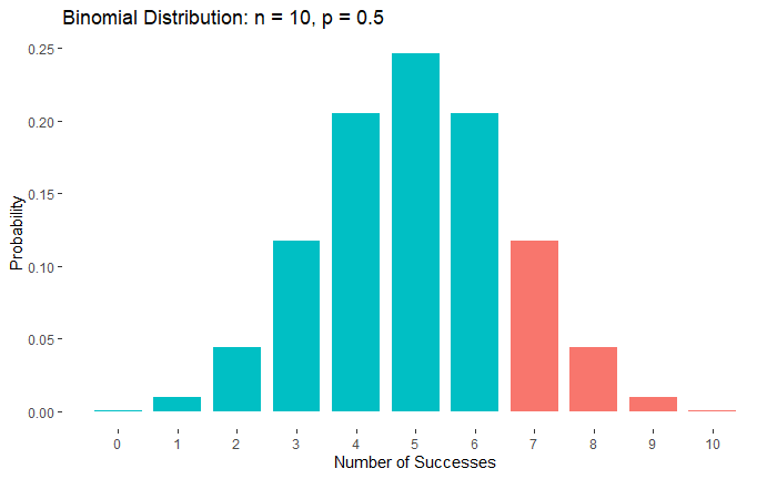
A person unexposed to statistics and random variations may conclude that at least five observations are required above 13.0 for the null hypothesis to be valid. And since there are only three, the null hypothesis is rejected. But we know about randomness and distributions, and therefore, ask this question: What is the probability of having seven negative observations from a binomial trial that is expected to have a 50% chance of success?

P(>=7) = P(7) + P(8) + P(9) + P(10) = 0.117 + 0.044 + 0.0098 + 0.001 = 0.172. In the following figure, it is the sum of the heights of the red bars.

So, the observations are unable to reject the null hypothesis. Before we end, answer this question: How many observations must be below 13.0 for the null hypothesis to be true? 

From the numbers and figure, it appears that you may need nine or ten observations below 13.0 for the sign test to make a rejection.

Does the magnitude of departure (from the median) play any role in rejecting the null hypothesis? We may have to explore another non-parametric test method, Wilcoxon signed rank, for that.

Non-parametric tests: zedstatistics

The sign test – Continued Read More »