October 2023

Dieing to Fill Glasses

Here is a game: There are six empty glasses – numbered 1 through six. You roll a die and fill an empty glass that matches the die roll. If the number on the die matches with an already-filled glass, it will be emptied. How many rolls are required to fill all six glasses?

Suppose there are five filled glasses, the number of die rolls required before the game ends is denoted by E(5). Based on this definition, E(0) must be the number of die rolls to finish the game starting with 0 filled glasses, equivalent to the original question.

E(5) = (1/6)[1] + (5/6)[1 + E(4) ]

E(4) must be in the following form to extend the logic.
E(4) = (2/6)[1 + E(5)] + (4/6)[1 + E(3) ]
E(3) = (3/6)[1 + E(4)] + (3/6)[1 + E(2) ]
E(2) = (4/6)[1 + E(3)] + (2/6)[1 + E(1) ]
E(1) = (5/6)[1 + E(2)] + (1/6)[1 + E(0) ]
E(0) = (6/6)[1 + E(1)]

Solving the five equations with five unknowns,

E(0) = 83.2

Reference

Can You Solve The Dice Rolling Drinking Game?: MindYourDecisions

Dieing to Fill Glasses Read More »
Contingency Tables – Continued

Contingency Tables are one way to organise data. Here is a data summary of computer users in a group.

PCMacRow
Totals
Male453883
Female405595
Column
Totals
8593178

Joint Probability

What is the joint probability of Female and Mac?
First, the answer: go to the cell at the junction of Female and Mac, i.e., 55 and divide by the total. 55/178 = 0.309.

Now the theory:
P (F AND Mac) = P(F | Mac) x P(Mac)
P(F | Mac) = 55/93
P(Mac) = 93/178
P (F AND Mac) = (55/93) x (93/178) = 55/178 = 0.309.

PCMacRow
Totals
Male45/178
= 0.25
38/178
= 0.21
Female40/178
= 0.22
55/178
= 0.31
Column
Totals

Conditional Probabilities

Conditional probability is the probability that an event occurs, given another event has happened. Given that a customer is female, what is the probability she’ll purchase a Mac?

The answer is female-Mac cell (55) and divide it with the female row total (95). 55/95 = 0.58.

PCMacRow
Totals
MaleP(P|M)
45/83
P(M|M)
38/83
83
FemaleP(P|F)
40/95
P(M|F)
55/95
95
Column
Totals
8593178
PCMacRow
Totals
MaleP(M|P)
45/85
P(M|M)
38/93
83
FemaleP(F|P)
40/85
P(F|M)
55/93
95
Column
Totals
8593178

Contingency Tables – Continued Read More »

Contingency Tables

Contingency Tables are one way to organise data. Here is a data summary of computer users in a group.

PCMacRow
Totals
Male453883
Female405595
Column
Totals
8593178

The intersection between the row and column defines one piece of information. For example, The intersection of PC and Male, 45, is the number of males (who participated in the survey) who use a PC at work, the junction between row total and females (95) is the total number of females in the survey, and a total of 178 people in the study, etc.

Marginal, Joint, and conditional probabilities 

Before we get into the calculations, a gentle reminder on probability.
P(event) = # Events / # Outcomes.

Marginal probabilities are the probabilities for single events without counting the other events in the table.
P(Female) = # Females / # Grand Total = 95 / 178 = 0.53.
P(Mac sold) = # Mac / # Grand Total = 93/178 = 0.52.

Let’s redraw the contingency table with marginal probabilities now.

PCMacRow
Totals
Male83/178
0.47
Female95/178
0.53
Column
Totals
85/178
0.48
93/178
0.52
178/178
1.0

Clearly, the numbers are all sitting on the margins, hence the name.

We’ll see the other two probabilities in the next post.

Reference

Statistics By Jim: Page

Contingency Tables Read More »

Chi-Square Distribution

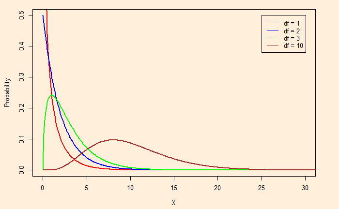
Chi-Square is a family of continuous distribution, widely used in hypothesis tests. The shape of a chi-square distribution is determined by what is known as the degree of freedom (df).

A chi-square test operates by comparing the observed distribution to what you expect if there is no relationship between the categorical variables.

Chi-Square Distribution Read More »

Likelihood Function – Part II

In the previous post, we estimated the likelihood of getting six people sick for two parameters (prevalence), 7% and 8%. We can also calculate the ratio between the two likelihoods:

L(theta = 0.07 | data = 6) / L(theta = 0.08 | data = 6) = 0.153 / 0.123 = 1.24. 

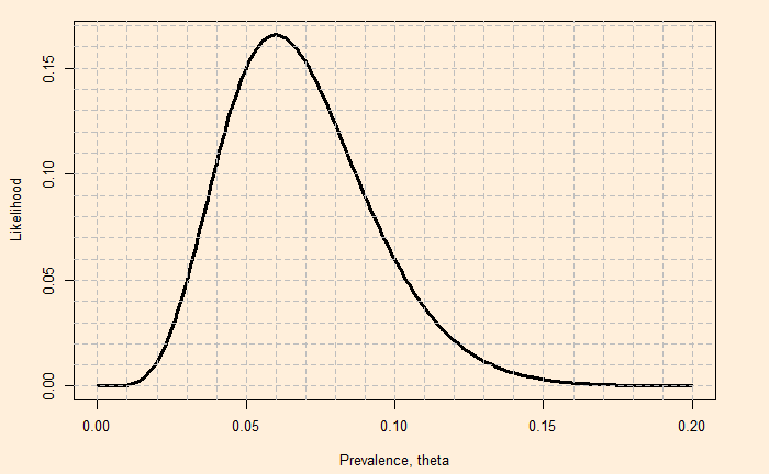
It means that the prevalence of 7% supports the data 1.24 times more than the prevalence of 8%. What about a sweep of likelihood over the entire parameter space? The function that gives the distribution of likelihoods of all possible values of parameters for a given data is the likelihood function.

As the parameter (theta) defines a model (e.g., binomial probability mass function), what the likelihood function is telling us is, given I have this data, what is the chance that the given model is true? In other words, we want the model that is mostly to have produced our data.

Likelihood Function – Part II Read More »

Likelihood Function

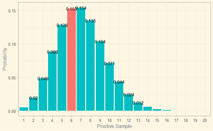
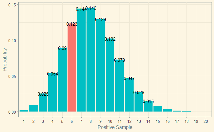
Consider two possible prevalence values for a rare disease, 0.07 and 0.08, respectively. If 100 samples from each city are taken, and six people are found positive, which prevalence value is likely?

Let’s visualise the situation 1:

And the situation 2:

It is clear that the first possibility, the prevalence (‘the parameter’) 0.07, is more likely, given 6 people tested positive as probability = 0.153 for the first case is > 0.123 for the second.

Summarising: for the parameter of 7%, the probability of getting six out of a hundred is 0.153. It becomes the likelihood.
L(theta = 0.07; y = 6) = 0.153 and L(theta = 0.08; y = 6) = 0.123

Here is the R code that generated the plot in situation 2.

xx <- seq(1,20)
P <-  dbinom(xx, 100, prob = 0.08)
binom_data <- data.frame(xx, P)

binom_data %>%  ggplot(aes(x=xx, y=P, label=P, fill=factor(ifelse(xx==6,"Highlighted","Normal")))) +
  geom_bar(stat="identity", show.legend = FALSE) +
  geom_text(aes(label=factor(ifelse(P > 0.01, round(P, 3),"")))) +
  scale_x_discrete(name = "Positive Sample", limits=factor(seq(1, 20, 1))) +
  scale_y_continuous(name = "Probability") +
  theme_solarized(light = TRUE) 

Likelihood Function Read More »

Period Life Expectancy – Plots

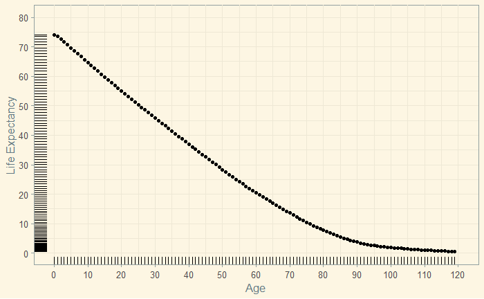
We have seen the calculations behind life expectancy, the lifespan of a hypothetical cohort ageing based on the measured mortality rates of a given period, as a statistical projection of the current conditions. Here, we plot the life expectancy that we estimated previously.

library(tidyverse)
library(ggthemes)
L_data %>% ggplot(aes(Age, Life.Exp)) +
geom_point() +
   geom_rug() +
  scale_x_continuous(name="Age", limits=c(0, 120), minor_breaks = seq(0, 120, 5), breaks=seq(0, 120, 10)) +
  scale_y_continuous(name="Life Expectancy", limits=c(0, 80), minor_breaks = seq(0, 80, 5), breaks=seq(0, 80, 10)) + 
 theme_solarized(light = TRUE) 

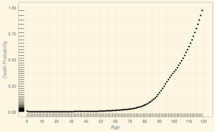
The death probability (data) at each age is presented below.

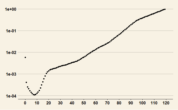
The plot with the Y-axis in the logarithmic scale shows finer details, especially in the lower age categories.

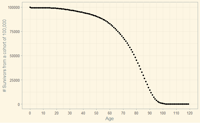
You can see below the dynamics of survival – 85,000 of the 100,000 are alive until almost the age of 60.

Period Life Expectancy – Plots Read More »

Period Life Expectancy

The period-life expectancy at a given age is the average remaining number of years expected for a person at that exact age, estimated from the mortality rate of that particular time. Let’s work out the calculation using the death probability (probability of dying within one year) table. The death probability is estimated from the mortality rates at each age (from census data for a short period). Here are the first few lines of the data (for complete data, see reference).

AgeP (Death)
00.005837
10.00041
20.000254
30.000207
40.000167

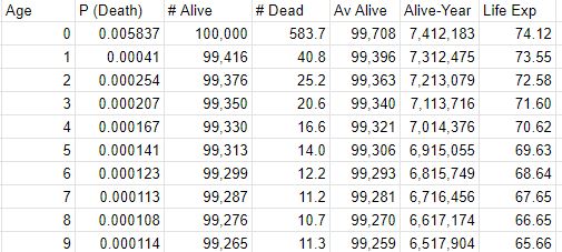
We start with 100,000 people in the cohort. The number of deaths in a given year, Yx = the probability of death (in Yx) x people alive (in Yx). In our example, for Y1, it is 100,000 x 0.005837 = 583.7.

The number of people alive in the next year (Yx+1 ) = people alive (in Yx) – the number of deaths in a given year (x). I.e., # Alivex+1 = 100,000 – 583.7 = 99,416. This number multiplied by the probability gives the number of dead in Yx+1.

The next step is to calculate the average number of people alive in the age category. It can be calculated as a mid-point average of the number of people in Yx+1 + (1/2) of the death in Yx. That equals 99,416 + 0.5 x 583.7 = 99,708.

In the next step, the total number of person-years lived by the cohort from age x until all cohort members have died. It is the sum of the numbers in the mid-point average column from age x to the last row in the table. Suppose there are a total of 120 columns (age numbers), and you want to calculate the person-years of age 24, you add all average alive from Y24 till Y119.

Life expectancy for a given age = person-years / persons alive.

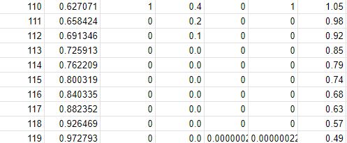
Here are the first and the last 10 years of calculations of a table that has 120 rows (Y0 – Y119).

References

Actuarial Life Table: SSA

The Life Table: lifeexpectancy.org

Period Life Expectancy Read More »

Likelihood Ratio – Fagan’s Nomogram

We have seen the likelihood ratio as the property of a diagnostic tool. Let’s take the fictitious screening tool we evaluated in the last post with LR+ = 10.7. Imagine a patient comes to a clinic with a few symptoms of a disease with a prevalence of 0.1 (very likely, age-adjusted), and this screening is a possible option. Would you recommend this? Note that the doctor will decide on further (costly) treatment only if she gets a conformation (posterior probability) of > 50% chance of the disease.

From the relationship we derived last time, 

OR_Post = LR x OR_Pri

Odds ratio (posterior) = 10.7 x 0.11 = 1.07
P(poterior) / (1 – P(poterior)) = 1.88
1/P(poterior) = 1 + 1/1.88
P(poterior) = 1.88/2.88 = 0.54

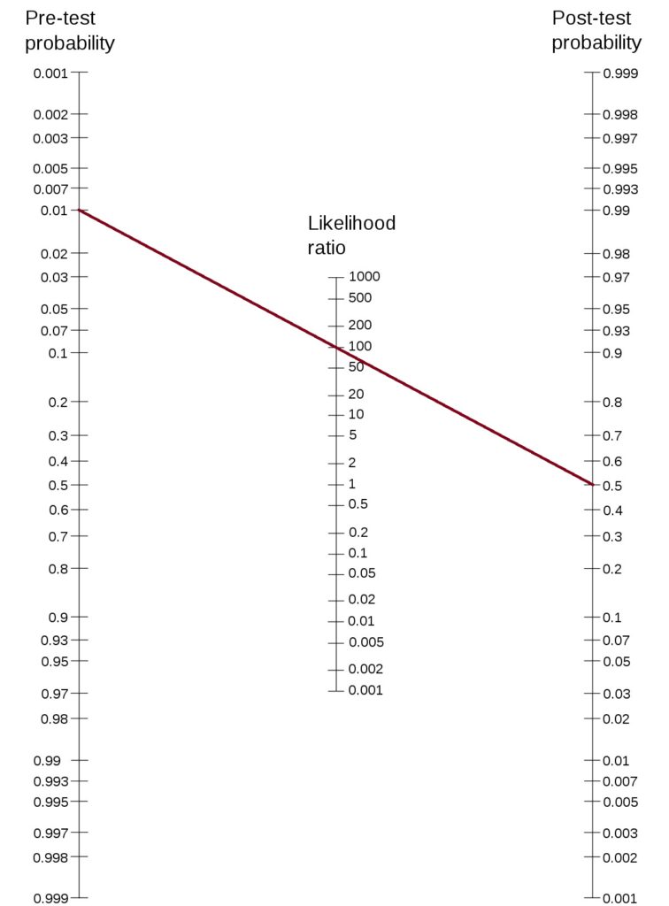
A nomogram of the following type is built to make such calculations simpler.

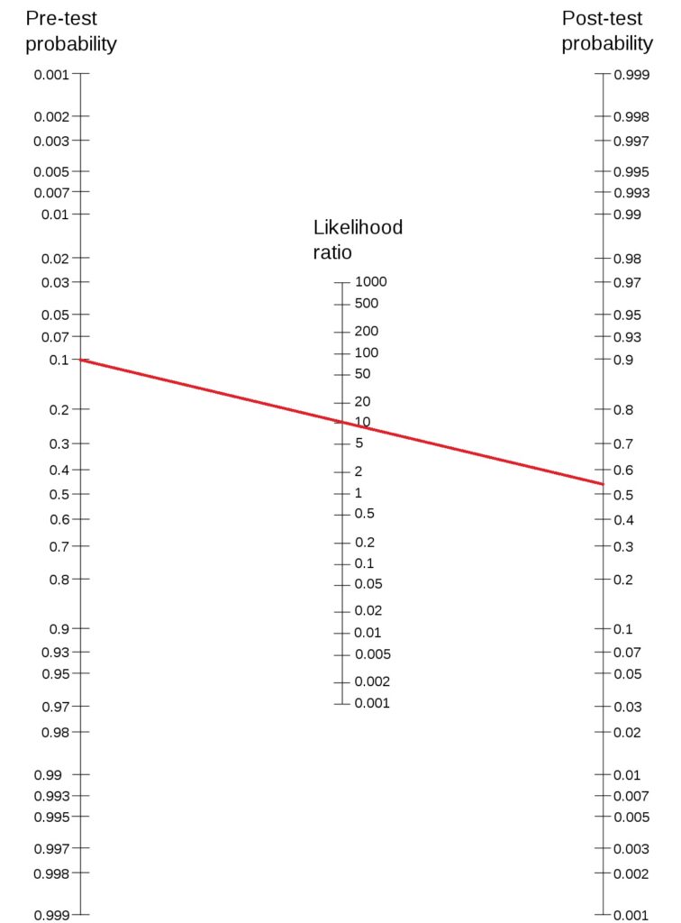
Draw a line from the ‘pre-test probability’ to ‘the likelihood ratio’ and extend it to the ‘post-test probability line. The intersection gives the posterior probability.

Here is an illustration of the method. Let’s use Fagan’s nomogram for the previous case,

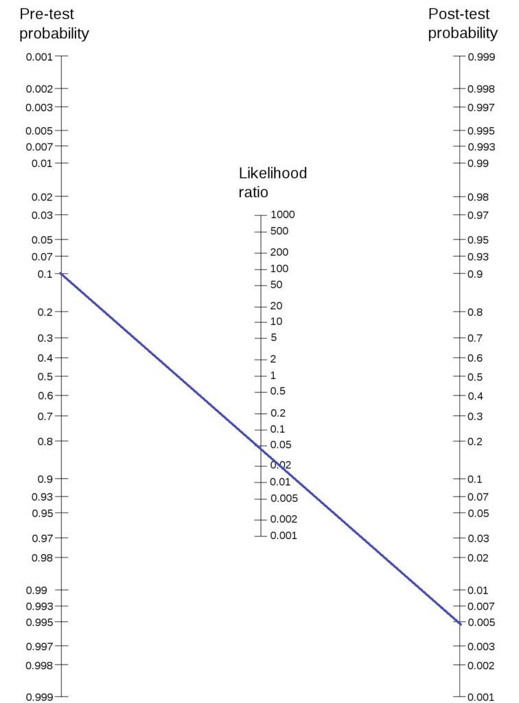
To answer the original question: this test may be recommended as it can bring the probability over 0.5 if the test comes positive. Not to forget, if the test comes negative (LR- = 0.044), the posterior probability becomes 0.005.

Smaller prior

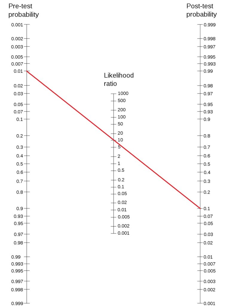
On the other hand, if the prior probability is lower, say, 0.01, as you can see below, the test is not very useful to make a conclusive decision.

Such a disease would require a diagnostic tool with a likelihood ratio of 100 or above to make a decision. Connect 0.01 (prior probability) to 0.5 (minimum decision criterion) and find out the likelihood ratio.

Likelihood Ratio – Fagan’s Nomogram Read More »

Likelihood Ratio and Posterior Odds

We know how the updated (posterior) disease probability is related to the prevalence (prior) via Bayes’ relationship.

\text{Posterior} = \frac{Sensitivity *  Prior}{Sensitivity *  Prior + (1-Specificity)*(1- Prior)}

Here, the ‘posterior’ and ‘prior’ are probability values. The corresponding odds ratio may be calculated using the following formula,

\text{Odds Ratio} = \frac{P}{1-P}

Using this definition, we estimate the odds ratio of the posterior as:

\\ OR_{post}= \frac{Posterior}{1-Posterior} \\ \\ = \frac{\frac{Sensitivity *  Prior}{Sensitivity *  Prior + (1-Specificity)*(1- Prior)}}{1 - \frac{Sensitivity *  Prior}{Sensitivity *  Prior + (1-Specificity)*(1- Prior)}} \\ \\ = \frac{Sensitivity *  Prior} {(1-Specificity)*(1- Prior)} = \frac{Sensitivity} {(1-Specificity)}\frac{Prior}{(1- Prior)}}

Notice the two terms: the first term, Sensitivity / (1 – Specificity), is the likelihood ratio and the second term, Prior / (1-Prior), is the odds ratio of the prior. Therefore,

OR_Post = LR x OR_Pri

Example

A new diagnostic tool yielded the following results.

  • A total of 1,000 individuals took the test.
  • 435 individuals had positive results, and 565 were negative.
  • Out of the 435 positive, 381 of them had the disease.
  • Out of the 565 negative, 549 did not have the disease.

What is the positive likelihood ratio of the test method?

From the data, true positives (TP) are 381. Then 435 – 381 = 54 must be false positives (FP).
Similarly, the true negatives (TN) are 549. 565 – 549 = 16 must be false negatives (FN).

Sensitivity = TP/(TP + FN) = 381/(381+16) = 0.96
Specificity = TN/(TN+FP) = 549 / (549 + 54) = 0.91

The likelihood ratio, therefore, is,
0.96 / (1 – 0.91) = 10.7

Likelihood Ratio and Posterior Odds Read More »