September 2023

Dice Polynomial – Sicherman Dice

September 10, 2023

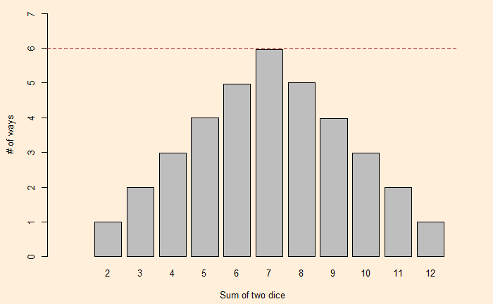
We have seen how one can describe a die with a polynomial. As a well-known example, i.e., the roll of two (regular) dice. The expected probabilities on the sum of dice are:

f(x) x f(x)= (x⁶ + x⁵ + x⁴ + x³ + x² + x¹) (x⁶ + x⁵ + x⁴ + x³ + x² + x¹)

x¹²+ 2x¹¹ + 3x¹⁰ + 4x⁹+ 5x⁸ + 6x⁷ + 5x⁶+ 4x⁵ + 3x⁴ + 2x³+ x²

Where the exponents of x are the X-values and coefficients of x are the Y-values.

Now, a question arises: Can we find another pair of two dice with the same distribution for the sums? One way to find out is to factorise the polynomial, x¹² + 2x¹¹ + 3x¹⁰ + 4x⁹ + 5x⁸ + 6x⁷ + 5x⁶ + 4x⁵ + 3x⁴ + 2x³ + x². George Sicherman discovered that another pair of numbers can lead to the same outcome. They are:

f(x) x g(x)= (x⁴ + x³ + x³ + x² + x² + x¹) (x⁸ + x⁶ + x⁵ + x⁴ + x³ + x¹)

They represent two cubes with the following numbering.
Cube 1: 1, 2, 2, 3, 3, 4
Cube 2: 1, 3, 4, 5, 6, 8

Let’s roll these dice a million times and find out.

dice_1 <- c(1, 2, 2, 3, 3, 4)
dice_2 <- c(1, 3, 4, 5, 6, 8)
prob_1 <- rep(1/6,6)
prob_2 <- rep(1/6,6)

itr <- 1000000

toss <- replicate(itr, {
sam1 <- sample(dice_1, 1, prob = prob_1, replace = TRUE)
sam2 <- sample(dice_2, 1, prob = prob_2, replace = TRUE)
sam <- sam1 + sam2
})

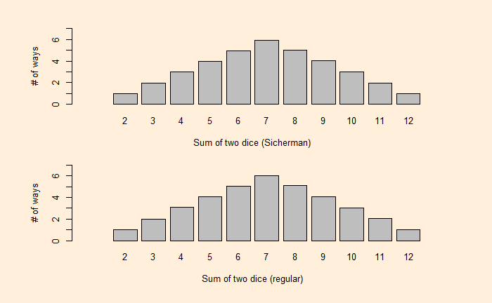
Here is the comparison of a pair of Sicherman dice with the regular.

Dice Polynomial – Sicherman Dice Read More »

What’s Wrong with the Fuel Standards?

September 9, 2023

Well, I don’t think there is anything wrong with it! They are like the carbon tax and the cap and trade – means to charge the emitter their share of the social cost of carbon.

But what are fuel standards? These are regulations set by the government targeting to cut down CO₂ emissions. For example, the US CAFE standards (corporate average fuel economy) required each manufacturer to meet two specified fleet average fuel economy levels for cars and light trucks, respectively. California pioneered the low carbon fuel standard that regulates the average carbon content per gallon of gasoline. If the former controls the amount one can burn, the latter focuses on capping the CO₂ in the given amount of fuel.

Let’s understand how a fuel efficiency standard operates.

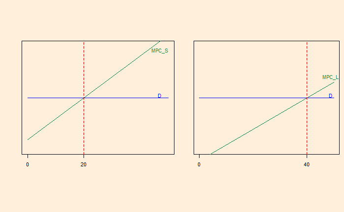
Suppose a manufacturer sells 20 small cars (S) and 40 large cars (L). Let the economies of these cards be 30 miles per gallon (mpg) for S and 10 mpg for L. The administration requires the average mpg (of the car sold) to be 20 mpg. On a simplistic level, this allows the company to sell one S for every L [(30 + 10) / 2 = 20 mpg]. Let’s look at a simplified supply-demand curve.

^{MPC = Marginal Private Cost or the change in the producer’s total cost brought about by the production of an additional unit. The flat demand curve means it is perfectly competitive.}

Naturally, this must change as per regulation because the average mpg is (20 x 30 + 40 x 10) / 60 = 16.7; less than 20. One solution is to reduce L production to 20 and bring the mpg to the compliance level.

The shaded triangle on the right is the amount of profit that is forfeited in this exercise. What happens if I sell five more Ls? It would mean the company must sell five more Ss at a loss.

This process can go on until the red-shaded area on the left matches with the green-shaded area on the right. That means the S car sales increase.

So, a performance standard subsidises the product, which makes the standard easier. In other words, the firm taxes the poor-performing car by subsidising the better performer. The plot will tell you that L is sold at a price higher than its marginal cost, whereas S is sold below its marginal cost.

So, what is wrong with fuel standards? There is a possibility that the firm ends up selling more cars than it would do otherwise. There is also a possibility for the Jevons paradox, where people end up driving the fuel-efficient car more (rebound).

What’s Wrong with the Fuel Standards? Read More »

Derangements

September 8, 2023

If n letters are placed randomly into n envelopes (with address), what is the expected number of envelopes with the correct letter inside?

Before addressing that, let’s look at a derangement problem. It is the probability of no match. For n items, it is the number of derangements divided by the number of permutations.

!n/n! = (n!/e)/n! ~ 1/e = 0.37

Let’s do a Monte Carlo and see what we get

itr <- 100000

let_env <- replicate(itr, {
  
  n <- 100
  
  env <- seq(1:n)
  let <- sample(seq(1:n), n, replace = FALSE, prob = rep(1/n, n))

  counter <- 0
for (i in 1:n) {
  if(env[i] == let[i]){
    counter <- counter + 1
  }else{
    counter <- counter 
  }
}

  if(counter == 1) {
    sounder <- 1  
  }else{
    sounder <- 0
  }
  

})

mean(let_env)

0.36827

So what about the original question of the expected number?

itr <- 100000

let_env <- replicate(itr, {
  
  n <- 100
  #env <- sample(seq(1:n), n, replace = FALSE, prob = rep(1/n, n))
  env <- seq(1:n)
  let <- sample(seq(1:n), n, replace = FALSE, prob = rep(1/n, n))

  counter <- 0
for (i in 1:n) {
  if(env[i] == let[i]){
    counter <- counter + 1
  }else{
    counter <- counter 
  }
}
  
 counter 
})

mean(let_env)

 1.00014

Derangements Read More »

Entropy and Information

September 7, 2023

We have seen how the entropy of a system is derived as the surprise element of a system. The higher the entropy, the higher the surprise, ignorance or the degree of disorder of the system.

As an extreme example, the entropy of a double-headed coin is zero as it contains no information, i.e., always lands on heads!

$\\ H = \sum\limits_{x=0}^{n} p(x) log_2[\frac{1}{p(x)}] \\\\ = 1 * log_2[\frac{1}{1}] + 0 * log_2[\frac{1}{0}] = 0$

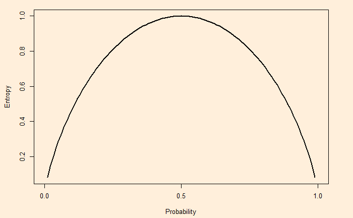
On the other hand, a fair coin (50-50) produces a non-zero entropy. The full spectrum of entropy for a coin toss is:

Entropy and Information Read More »

The Surprising Story of Entropy

September 6, 2023

Entropy is a concept in data science that helps in building classification trees. The concept of entropy is often explained as an element of ‘surprise’. Let’s understand why.

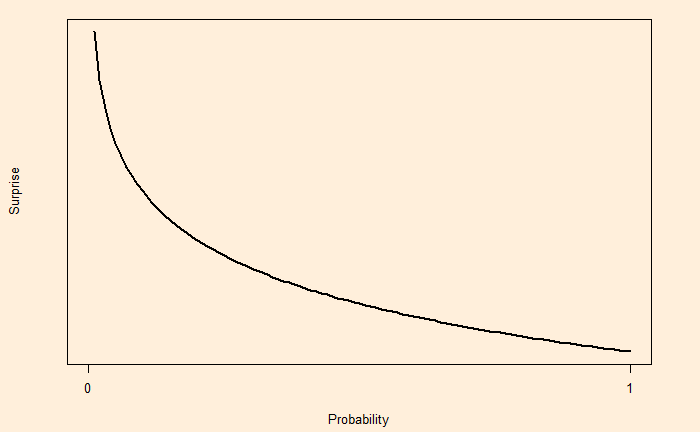
Suppose there is a coin that falls on heads nine out of ten or the probability of heads, p(H) = 0.9. So, if one tosses the coin and gets heads, it is less of a surprise as we expect it to show this outcome more often. whereas when it shows a tail, it is more surprising. In other words, surprise is somewhat an inverse of the probability, i.e. S = 1/p. But that has a problem.

If the probability of something is 1 (100% certain), 1/p becomes 1/1 = 1. Since we know the chance of that outcome is 100%, it should not be a surprise at all, but we get 1. To avoid that situation, S is defined as log (1/p).
p = 1; S = log (1/1) = 0.
On the other hand,
p = 0; S = log(1/0) = log(1) – log(0) = undefined.

It is a practice to use log base 2 for calculating surprise for two outputs.

Surprise = log₂(1 / Probability)

Now, let’s return to the coin with a 0.9 chance of showing heads. The surprise for getting heads is log₂(1/0.9) = 0.15 and log₂(1/0.1) = 3.32 for tail. As expected, the surprise of getting the rarer outcome (tails) is larger.

If the coin is flipped 100 times, the expected value of heads = 100 x 0.9 and the expected value of tails = 100 x 0.1.
The total surprise of heads = 100 x 0.9 x 0.15
The total surprise of tails = 100 x 0.1 x 3.32
The total surprise = 100 x 0.9 x 0.15 + 100 x 0.1 x 3.32
The total surprise per flip = (100 x 0.9 x 0.15 + 100 x 0.1 x 3.32)/100 = 0.9 x 0.15 + 0.1 x 3.32 = 0.47

This is entropy – the expected value of the surprise.

The Surprising Story of Entropy Read More »

Climate Change – Pew Research Survey

September 5, 2023

Motivated reasoning is the tendency to favour conclusions we want to believe despite substantial evidence to the contrary. A famous example is climate change. In the US, for example, Democrats and Republicans disagree on the scientific consensus. A recent Pew Research survey on climate change presents the magnitude of this divide.

Prioritise alternative energy

At the highest level, 67% of people support this view, which is pretty impressive. But that is 90% Democrats (and Democrat-lining) and 42% Republicans (and leaning). The only silver lining is that 67% of Republicans under age 30 support alternative energy developments.

Climate change – a major threat to the well-being

Here again, the difference between the two parties is stark. In the last 13 years, the views from the Democrats have steadily increased from 61% to 78%, acknowledging climate change as a major threat. It has remained steady and low for the Republicans – at 25% in 2010 and 23% in 2022.
Interestingly, 81% of French and 73% of Germans regard it a threat.

Americans’ views of climate change: Pew

Climate Change – Pew Research Survey Read More »

A Vegan View of Health

September 4, 2023

The Netflix documentary, ‘What the Health’, may belong to a class of faulty reasoning known as propaganda. Let’s look at some of the logical fallacies committed by the program.

The documentary intends to promote Veganism, which, I think, is fair. Food accounts for about 25% of greenhouse gas emissions, of which meat occupies half. However, the tactics used by the producer of the film range from cherry-picking to total misinformation.

Meat and cancer

The program begins with the infamous connection between processed meat and (colorectal) cancer, which comes from the 2015 findings in the International Agency for Research on Cancer (IARC). One main suspect is the production of polycyclic aromatic hydrocarbons (PAHs) during cooking by panfrying, grilling, or barbecuing. This has led to the classification of processed meat in Group 1 (Carcinogenic to humans) and red meat in Group 2A (Probably carcinogenic to humans) as per IARC.

Statistics of the low base

We already know the background of the study and what an 18% increase means. In simple language, the average prevalence of colorectal cancer (5 in 100) becomes 6 for meat eaters. As a comparison, smoking makes the lifetime risk of lung cancer 17.2 in 100 vs. 1.3 in 100 for non-smokers – a 1000% increase.

Appeal to fear

The program also chooses some of the fellow 126 candidates, such as Plutonium, Asbestos and cigarettes, to emphasise the seriousness of Group 1. On the other hand, it conveniently forgets that alcoholic beverages, areca nuts and solar radiation are a few other items on the same list. To reiterate, the items in one group do not have the same risk. A place in Group 1 only means the association (with cancer) is established for that item and nothing about the absolute risk.

Sugar-coated binary

The film then argues with the help of a few ‘experts’ that sugar, considered many as a problem molecule, plays no role in diseases such as diabetes. Such creation of the innocent-other to demonise the intended subject was totally unnecessary.

Missing the balances

The documentary slips into propaganda because it misses the balance. There is no debate here about the need to incorporate more plant-based diet and exercise in the lifestyle. It is also important to have the right amount of micronutrients and protein in the diet, which may include meat, egg and dairy products.

The documentary is propaganda as it primarily appeals to emotion. The objective is to form opinions rather than increase knowledge. It uses strategies such as cherry-picking, appealing to fear and misinformation.

References

IARC Report on Processed Meat

Known Carcinogens: Cancer.org

Carcinogenicity of Processed Meat: The Lancet Oncology

How common is colorectal cancer: cancer.org

Carbon Footprint Factsheet: umich

Climate change food calculator: BBC

IARC Classifications: WHO

IARC Group 1 Carcinogens: Wiki

Lung cancer by smoking: Pub Med

A Vegan View of Health Read More »

Birthday Problem – Data

September 3, 2023

We have seen the birthday problem earlier, and a group of 23 has a 50% chance that two of its members will share a birthday. Here is a real test to validate it. We use birth data from the recently concluded women’s World Cup. The data is available in the reference.

The following R code arranged the data of 736 players that belonged to 32 teams.

F_data <- read.csv("D:/Misc/DataData/Footer1.csv")
F_data <- as.data.frame(matrix(F_data$DOB, nrow = 23))
names(F_data) <- paste0("TEAM", 1:ncol(F_data))
as_tibble(F_data)

The next set of calculations modifies the dataset into a month-date format.

F_data1 <- F_data
for (i in 1:ncol(F_data)) {
  F_data1[,i] <- as.Date(F_data[,i], format = "%d/ %m/ %Y")
  F_data1[,i] <- format(F_data1[,i], format="%m-%d")
}
as_tibble(F_data1)

The final set of codes calculates if any date is duplicated in each team and gets the total number of such instances.

match1 <- rep(0, ncol(F_data1))
for (i in 1:ncol(F_data1)) {
match1[i] <- any(duplicated(F_data1[,i]) == TRUE)
}

match1
sum(match1)

0 0 1 1 0 1 1 1 0 1 1 1 0 1 0 0 1 0 0 1 1 1 0 0 0 1 0 0 0 1 1 1 

17

Since for a 23-member group, there is a 50% chance. Therefore, in a 30-team competition, the expectation is 16 teams on average. And in reality, it turned out to be 17; not bad, eh?

Reference

Squad List: women’s world cup

Birthday Problem – Data Read More »

Bayesian Snow Flakes

September 2, 2023

Alice says there was snowfall last night. Becky says Alice lies 5 out of 6 times. Carol checked the previous day’s weather prediction and said the probability of snow was 1/8. What is the probability that there was snow?

We will use Bayes’ theorem to get the answer:

P(SN|AS) – Probability that it snowed, given Alice said so.
P(AS|SN) – Probability that Alice said snowed, given there was snow.
P(SN) – Prior probability of having snow.
P(AS|NS) – Probability that Alice said snowed, given there was no snow.
P(NS) – Prior probability of having no snow.

$\\ P(SN|AS) = \frac{P(AS|SN)*P(SN)}{P(AS|SN)*P(SN) + P(AS|NS)*P(NS)} \\ \\ \frac{(1/6)(1/8)}{(1/6)(1/8) + (5/6)(7/8)} = \frac{1}{36}$

1/36

Bayesian Snow Flakes Read More »

Probability of Double Dice – Convolution

September 1, 2023

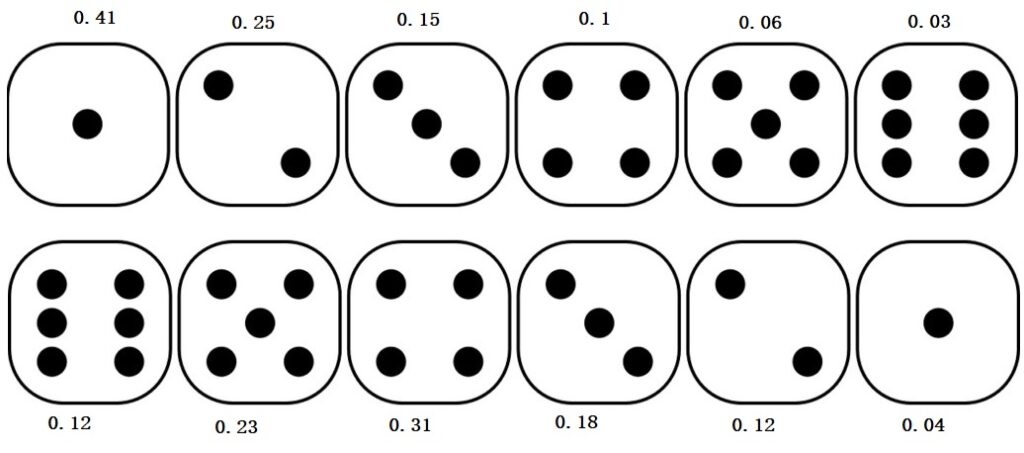
We have seen how the probability of double dice can be estimated by flipping and sliding the outcomes of the second die. Here is another example to illustrate the concept: this time, with two dice with different probabilities.