April 2023

Singing Competition

Ana, Becky and Claire are three singers entering a contest. Ana has won 4% of past competitions, Becky has 5%, and Claire has 6%. If Ana has submitted 7 albums, Becky 2 and Claire 3, what is the probability that Ana will win this time?

The general formula of Bayes’ theorem is:

\\ P(j|W) = \frac{P(W|j)*P(j)}{\sum\limits_{i = 1}^{n} P(W|i)*P(i)} \\ \\ \frac{P(W|j)*P(j)}{P(W|1)*P(1) + P(W|2)*P(2) + P(W|3)*P(3)}

In the present case, for Ana, it is:

\\ P(Ana|W) =  \frac{P(W|Ana)*P(Ana)}{P(W|Ana)*P(Ana) + P(W|Becky)*P(Becky) + P(W|Claire)*P(Claire)} \\\\ \frac{0.04 *(7/12)}{0.04 *(7/12) + 0.05 *(2/12) + 0.06 *(3/12)} = 0.5

50% chance!

Singing Competition Read More »

The Dropout Fallacy

Why do people go to college? To some, it is to learn. To academics and philosophers, it is more than just learning to enrich intellectual and social capital in individuals. But to many, a college education prepares them to get a job.

And there is nothing wrong with that thought – there is a strong positive correlation between jobs and education. Here is data from the U.S.  Bureau of Labor Statistics: 

Degree Median
Salary (USD)
Unemployment
Rate (%)
Doctoral 19091.5
Professional 19241.8
Master’s15742.6
Bachlor’s13343.5
Associate’s9634.6
College, no degree8995.5
High School8096.2
Less than
High School
6268.3
Unemployment Rates and Earnings by educational attainment, 2021
Note: Data are for persons aged 25 and over. Earnings are for full-time wage and salary workers.
Source: Current Population Survey, U.S. Department of Labor, U.S. Bureau of Labor Statistics

But only until you encounter the superheroes – the Gates, the Dells and the Jobs – the college dropouts! The countless stories and speeches reinforce the theme that dropouts counterbalance their short-coming in education through their determination, superior intelligence and perseverance.

There can be a lot of factors behind the observation of successful dropouts. Foremost among them is randomness: out of the millions that have a chance but fail to complete their college, a negligible few happen to become millionaires. And they get more airtime in public. In that respect, the dropout fallacy is a survivorship bias.

The second invisible factor is related to the confounding effect of the social and cultural capital of the prosperous – such as access to a network of successful people, easy access to financing their ventures etc.

References

Unemployment Rates and Earnings by educational attainment, 2021: U.S. BLS
The Myth of the Successful College Dropout: The Atlantic

The Dropout Fallacy Read More »

Free and Unlimited

The concept of FREE! is one of the most compelling forces on human irrationality. Based on many examples, it has been proven that the market power of FREE! is not an extrapolation of discount.

In a famous experiment by Shampanier et al., the researchers offered to the participants a choice between Hershey’s (low-value chocolate) and Lindt truffle (high-value) for three different price offers – (0&14), (1&15) and (0&10). The first number inside the bracket refers to the price of Hershey’s in cents, and the second is that of Lindt. And the results showed the demand for Lindt dropped from 36% to below 20% in both the FREE! options and that of Hershey’s went up from 14% to 40%. Note that 40-50% of the participants opted for nothing.

In the real world, the appeal to free and unlimited has been hailed as a blockbuster success story behind India’s Jio telecom company. When it was launched for the public in September 2016, Jio SIM cards were available for free, along with 4GB of data a day, for three months. And the results? The Indian telecom industry, which had six players at that time, was reduced to four, and Jio captured about 350 million subscribers today.

Dan Ariely, Predictably Irrational

Shampanier et al., Zero as a Special Price: The True Value of Free Products, Marketing Science, 26 (6), 2007, 742

Free and Unlimited Read More »

News From Huanan Market

After a brief interval, here is some Covid news. A new peer-reviewed article is now available in Nature for preview. The study summarises the RNA sequence results from several samples from Huanan Seafood Market in Wuhan. The market was linked to several of the early cases of the illness. Since the market’s closure (1st of January 2020), 923 environmental and 457 animal samples were collected from 1-Jan to 2-Mar 2020. Here is the high-level summary:

# Samples# +ve by
RT-PCR
Huanan Seafood Market71840
Warehouses145
Other markets301
Drainage11024
Sewerage wells513
Total92373
Summary of environmental sample results

Notably, 35 samples from February showed positive, suggesting a pretty long persistence of the viral material in the environment.

Of the 457 samples collected from animals belonging to 18 species, none of them tested positive for the virus.

While several samples had genetic material belonging to mammals of genera such as homo (e.g. human), ovis (e.g. sheep), bos (e.g. cow), canis (e.g. dog) etc., it is not, however, proof that these animals were infected but may only mean that there was an increased focus (for sample collection) on those shops and locations, where animals were sold. The same goes with the case of racoon dogs as carriers: the study found genetic material from those; it could only mean that two things (virus-carrying entity and racoon dogs) co-existed, and nothing further.

Reference

Surveillance of SARS-CoV-2 at the Huanan Seafood Market: Nature

News From Huanan Market Read More »

Rare Disease Revisited

Remember when we discussed the application of Bayes’ theorem to quantify the predictive values of medical tests? It gives the probability that a person has a (rare) disease, given she is tested positive. Today, we verify the solution using a simple R code by sampling a million people!

Using the familiar notations, we write down Bayes’ formula.

P(D|+) = \frac{P(+|D) P(D) }{P(+|D) P(D) + P(+|NoD) P(NoD)}

Let’s assign probabilities to each of the parameters.

1) The test shows positive 90% of the time on patients with the disease (high sensitivity); P(+|D)
2) The test shows negative 95% of the time on healthy patients (high specificity); P(-|noD)
3) The disease is present in 1% of the community (low prevalence ) P(D)

Note that specificity = P(-|noD), whereas what we want is P(+|NoD), which is 1 – P(-|noD). Substituting all values,

\\ P(D|+) = \frac{P(+|D) P(D) }{P(+|D) P(D) + P(+|NoD) P(NoD)} \\ \\ P(D|+) = \frac{Sensitivity *  Prevalence}{Sensitivity *  Prevalence + (1-Specificity)*(1- Prevalence)} \\ \\ P(D|+) = \frac{0.9*0.01}{0.9*0.01 + 0.05*0.99} = 0.15

Let’s develop a code that simulates the testing of a million people.

Step 1: A million people, with 1% (random) having the disease. 1 = disease, 0 = no disease.

disease <- sample(c(0,1), size=1e6, replace=TRUE, prob=c(0.99,0.01))

Step 2: Create an empty vector with a million slots.

test <- rep(NA, 1e6)

Step 3: Fill the disease columns (disease = 1) with random assignment of test results; 90% with 1 and 10% with 0.
Fill the nondisease columns (disease = 0) with random assignment of test results; 95% with 0 and 0.05% with 1.

test[disease==1] <- sample(c(0,1), size=sum(disease==1), replace=TRUE, prob=c(0.1, 0.9))
test[disease==0] <- sample(c(0,1), size=sum(disease==0), replace=TRUE, prob=c(0.95,0.05))

Now estimate the average number of people with disease = 1 AND test = 1.

mean(disease[test==1]==1)

Putting everything together,

disease <- sample(c(0,1), size=1e6, replace=TRUE, prob=c(0.99,0.01))
test <- rep(NA, 1e6)
test[disease==1] <- sample(c(0,1), size=sum(disease==1), replace=TRUE, prob=c(0.1, 0.9))
test[disease==0] <- sample(c(0,1), size=sum(disease==0), replace=TRUE, prob=c(0.95,0.05))
mean(disease[test==1]==1)

Rare Disease Revisited Read More »

The Stupidity paradox

The stupidity paradox is a term introduced from the works of Mats Alvesson, Professor of Business Administration Mats Alvesson at Lund University, Sweden and Andre Spicer, Professor of organisational behaviour, City University London. As per the theory, functional stupidity is a state where employees in an organisation perform as expected but never question if they are doing the right thing or not.

As per the authors, the stupidity paradox happens when companies that claim to be knowledge-based recruit smart, educated staff but end up doing dumb things.

The Stupidity paradox Read More »

Five Laws of Stupidity

It comes from an article written by Carlo M. Cipolla in the 1970s. He puts forward five laws.

  1. Everyone underestimates the number of stupid people around you. It means people often get carried away by what they see from outside – education, race, eloquence etc.
  2. The probability of a person being stupid is independent of any other characteristic of that person. In other words, stupidity is uncorrelated with gender, nationality, wealth or education.
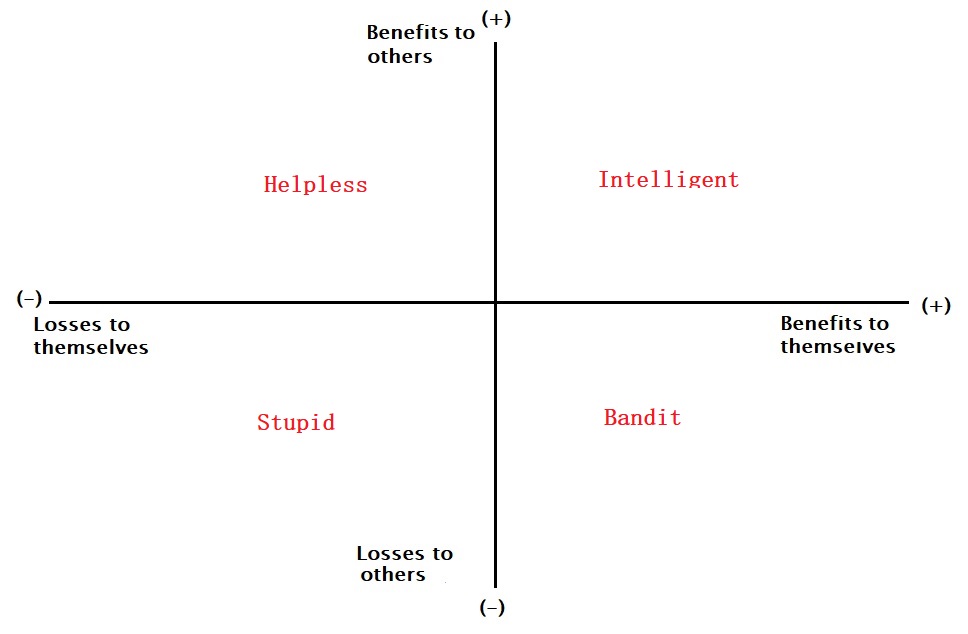
  3. The stupid person causes losses to others while deriving no gain and possibly incurring losses.
  4. Non-stupid people always underestimate the damaging power of stupid individuals.
  5. A stupid person is the most dangerous type of person

Cipolla built a 2 x 2 matrix to explain rule number 3.

Five Laws of Stupidity Read More »

The paradox of weak ties

In 1973, Mark Granovetter reported in a paper titled “the strength of weak ties” that acquaintance and weak ties are more effective – be it creativity or getting jobs. As a definition: strong ties are between densely knit close friends, whereas weak links are between people with infrequent interaction and a lack of any emotional connection. He hypothesised that the diversity of information and ideas inside the “diffused” network (as against close-knit groups) of people was responsible for such observations.

While it remained a paradox and got support from many subsequent studies, the confounding of two parameters – the number and the strength of bonds – was not apparent in these studies. A 2017 work that looked at 17 million social ties from Facebook users concluded that the usefulness of weak ties arises because of the sheer number. In other words, while the probability of getting something (a new idea or a job) helpful from weak connections may remain low, the numbers are overwhelmingly larger than strong relationships; the former get the overall advantage.

Granovetter, M. S., American Journal of Sociology, 1973, 78, 1360
Gee, L.K. et al. / Journal of Economic Behavior & Organization, 2017, 133, 362

The paradox of weak ties Read More »

IESDS – Infering Each Other

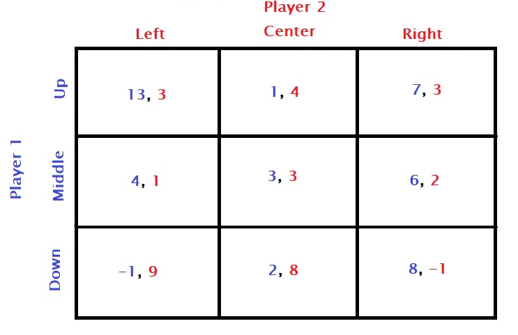
See a game played between two rational players with the following payoff matrix.

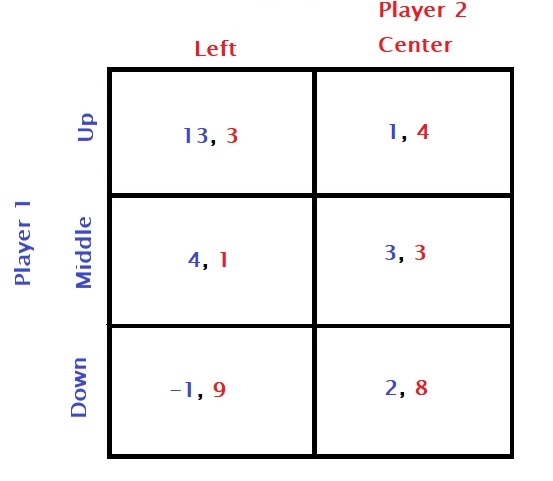
Looking at the matrix, one can see that player 2 is unlikely to choose the right strategy as her payoffs, 3, 2 and -1, are worse off against left and centre. So for player 2, the matrix is the following.

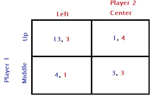
Player 1 knows what Player 2 is thinking because she is also rational. She looks at her options and concludes that down is no longer an option for her (- 1 < 4 and 2 < 3). So he eliminates the row corresponding to down.

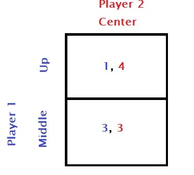
Player 2 knows that the option down is the least favourite to Player 1, so she compares options left and centre. Centre dominates (4 > 3 and 3 > 1).

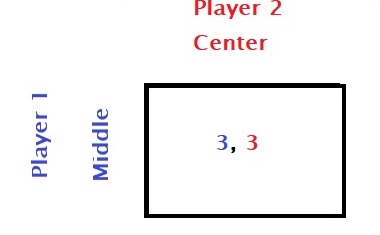
If that is the case, Player 1 will choose the middle, which gives her a better incentive.

The whole game structure is common knowledge between the two players. Such games are known as iterated elimination of strictly dominated strategies or IESDS.

IESDS – Infering Each Other Read More »

Strategies of a Game

Based on what we have seen so far, let’s put together three strategies for games we have encountered in the past. But before delving into those, look at Nash’s theorem, which suggests that there must be at least one Nash equilibrium in all finite games. Watch out for those two words: Nash equilibrium and finite games!

A finite game has a fixed number of players, a defined set of rules, and a known end.
Nash equilibrium is the state of a game where the player has made her best decision or has no incentive to change the decision, assuming all other players maintain their current strategy.

The dominant strategy

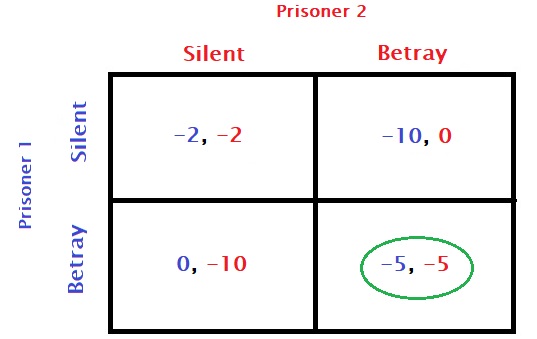
Remember the prisoner’s dilemma? The prisoner has a clear move irrespective of what the others will do. To put it in the language of the payoff matrix,

The pure strategy

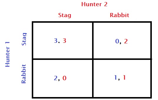
The stag hunt game;

Compare dominant and pure

In the first instance, they may appear the same: one best outcome, one sub-optimal and two places with mixed incentives. But look carefully: in the first game, imagine you are prisoner 1, and think about your reward (the blue number) based on the two possibilities of the other player. If prisoner 2 is silent (first column), then your choice is to betray as 0 > -2 (compare the two blue numbers of the first column). If prisoner 2 chooses to betray (second column), your choice is still to betray as -5 > -10 (compare the two blue numbers of the second column). 100% clarity!

In the second case, repeat the above process. If hunter 2 brings the tool for the stag, the stag becomes your choice (blue 3 > blue 2). If hunter 1 gets the rabbit device, the rabbit is your choice (blue 1 > blue 0).

The mixed strategy

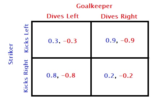
The penalty kick game is an example of a zero-sum game—one person’s win is the other’s loss. There is no pure strategy here; one needs to mix up (randomise) the plan to succeed. In other words, the strategy needs probabilistic estimation.

Strategies of a Game Read More »