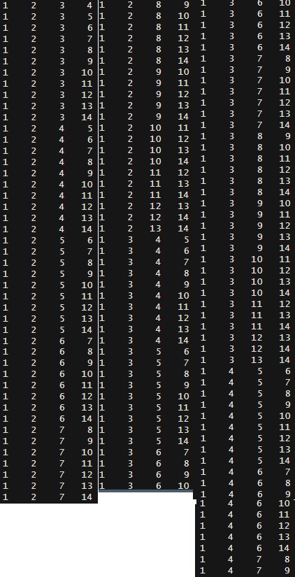
NBA Draft – Probabilities
Now that you know the probabilities given to the fourteen teams and how the lottery system works, what are the chances that team number 1 gets the lottery?
Getting first
What is the probability of team number 1 (the team with the worst performance in the regular season) getting the lottery in the first draw?

Getting second
What is the probability that Team 1 gets lucky in the second draw? Well, it is the joint probability that another team (i) obtains the first draw AND team 1 gets the second.

Notice X, the number of combinations allocated to team ‘i’ that won the first, will not be available for the second lot, and, therefore, you subtract from 1000. And remember, ‘i’ varies from 2 to 14 (all squads other than Team 1). So, you estimate the joint probability with each of them and add them up. Rearrange terms and sum it over ‘i’,

Let’s estimate the value using the R code:
prob_value <- c(0.14, 0.14, 0.14, 0.125, 0.105, 0.09, 0.075, 0.06, 0.045, 0.03, 0.02, 0.015, 0.01, 0.005)
prob.sum = 0
for(i in 2:14){
    current = prob_value[i]/(1-prob_value[i])
    prob.sum = prob.sum + current
}
prob.sum*prob_value[1]
The answer is 0.1341732. The probability of team 1 getting lucky in the first two draws = 0.14 + 0.1341732 = 27%
Getting third
Extending the same logic, the probability for Team 1 to get the third lot is

prob_value  <- c(0.14, 0.14, 0.14, 0.125, 0.105, 0.09, 0.075, 0.06, 0.045, 0.03, 0.02, 0.015, 0.01, 0.005)
prob.sum = 0
for(i in 2:14){
  for(j in 2:14){
    if(i != j){
          prob.sum =  prob.sum + prob_value[i]*prob_value[j]/ ((1-prob_value[i]) * (1-prob_value[i]-prob_value[j]))
      }
     }
  }
prob.sum*prob_value[1]
0.1274865. So, for team 1 getting in the first three draws = 0.14 + 0.1341732 + 0.1274865 = 40 %
Getting fourth (final)

prob_value <- c(0.14, 0.14, 0.14, 0.125, 0.105, 0.09, 0.075, 0.06, 0.045, 0.03, 0.02, 0.015, 0.01, 0.005)
prob.sum = 0
for(i in 2:14){
  for(j in 2:14){
    for(k in 2:14){
          if(j != k){
            if(i != j){
              if(i != k){
    current = (prob_value[i]/(1-prob_value[i])) * (prob_value[j]/(1-prob_value[i]-prob_value[j])) * (prob_value[k]/(1-prob_value[i]-prob_value[j]-prob_value[k]))
    prob.sum = prob.sum + current
              }

          }
    }
      }
  }
}
prob.sum*prob_value[1]
0.1197205. So, for team 1 getting one of the lotteries = 0.14 + 0.1341732 + 0.1274865 + 0.1197205 = 52.1 %
NBA Draft – Probabilities Read More »