waiting time paradox

Guys Finish Last

Do you remember the last time you were in a queue that reached the counter ahead of others who joined at similar times as you did? It could be a bit of a struggle to recollect, but I’m sure you remember the time you finished the last! Let’s analyse what must be happening with you.

Clue 1: Selective memory

The simplest explanation for your troubles is selective memory. Don’t you remember that day you wanted to write down a number in a phone call and found the pen was not working? You know it was not the first telephone you attended in life where you had to write something down. And you had a pen that worked, but you took it for granted – after all, the purpose of that device is to write.

You are more likely to recollect the days you finished last than you did first. And that is human nature. Biologists speculate this is part of an evolutionary defence mechanism that you remember the past incidents that led you to trouble, perhaps as a trigger not to repeat them.

Clue 2: Probability

We have seen several examples already. You are entering a billing section of a store that has ten lines. If you pick a random queue, what is the probability that you end up in the fastest? The answer is 1/10. To state it differently, what is the chance that you are not the fastest? Nine out of ten. Then you argue that it was not accidental and that you selected the shortest. There are two possible responses to that feeling.

First, all the others in the hall also (think they) selected the shortest, and your selection, regardless of how you felt, was still random. The second explanation concerns the specific information about your choice that you lacked and the others had. It was short as there was something in that queue – a slower attendant or people with items that required more time for the check-in. And you just took that. Once you are in the line and start measuring the average time taken by the others, you get into what is known as the inspection paradox.

Clue 3: WAITING-TIME PARADOX

We have seen it before in the name of the inspection paradox and waiting time paradox. We proved mathematically that the actual waiting time is longer than the theoretical average calculated based on the frequency of occurrences.

In short

Next time the feeling occurs on why it happened only to you and not anyone else, think again. It is more likely that the others, too, feel the same; after all, the “you” I chose in the description is just an arbitrary choice.

Reference

The formula for choosing the fastest queue: The conversation
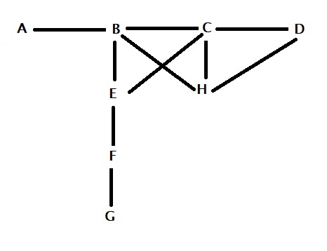
Guys Finish Last Read More »

The Weighted Average paradox

If there is one statistical feature that links all three topics we have discussed in the last three days, starting with the inspection paradox, it will be the weighted average. In simple terms, if you make a random attempt to make a selection, your choice will be over-represented by the heavies. Be it a survey on classes, connecting to friends on social media or the waiting time for buses.

Think about a fortune wheel as depicted below. It’s spinning fast, and you come and touch the surface to stop it. Based on the number inscribed on the section, you get points. Note that the area of the cell is proportional to the number.

Without this information, you would have assumed the (expected) average prize to be 100/5 = 20. But when you look at the figure, you notice that the chances of hitting the different sections are not equal but related to the number on the wheel. To repeat the phrase that we have started with – it is proportionally over-represented by the heavies.

The expected value must take the probabilities. And thefore, it becomes 0.4 x 40 + 0.05 X 5 + 0.20 x 20 + 0.25 x 25 + 0.1 x 10 = 27.5

The Weighted Average paradox Read More »

Friendship Paradox

You know, your friends, on average, have more friends than you do! I know it is a bit difficult to swallow that feeling. We will explore it mathematically. On the one hand, it follows from what we have seen before – the inspection paradox and the waiting-time paradox. But we will use a different approach here.

Count your friends

Consider the following relationship tree.

What it means is that A has only one friend (i.e., B) denoted by A(1; B). Similarly B(4; A, C, E, H), C (4; B, D, E, H), D(2; C, H), E(3; B, C, F), F(2; E, G), G(1; F), H(3; B, C, D). So the total number of friends among those eight is 1 + 4 + 4 + 2 + 3 + 2 + 1 + 3 = 20. The average number of friends, therefore, is 20/8 = 2.5.

And their friends

How do we do it? The easier way is to call out each of them and ask how many friends they have. For example, take A: she will ask her only friend, B, to call out her friends. B has four friends (note that it also includes A). Let us represent that as A{B(4)}. Similarly, B{A(1), C(4), E(3), H(3)}, C {B(4), D(2), E(3), H(3)}, D{C(4), H(3)}, E{B(4), C(4), F(2)}, F{E(3), G(1)}, G{F(2)}, H{B(4), C(4), D(2)}. The total number is 60. To calculate the average friends’ friends, you should divide 60 by the friends you calculated earlier, i.e., 20. 60/20 = 3.

So by counting, you prove that the average number of friends (2.5) is smaller than friends’ friends (3). The whole exercise can be summarised in the following table

IndividualFriends
(P)
Friends’ friends
(Q)
Mean
Friends’ friends
(P/Q)
A1 44
B4 112.75
C4123
D273.5
E3103.33
F242
G1 22
H3103.33
Total206023.91

Analytical Proof

Look at the diagram once more. We replace the number of friends that A have with dA (dA represents the degree of the vertex that points from person A).

\\ \text{In other words, the total number of friends here is }, \\\\ d_A + d_B + d_C + d_D + d_E + d_F + d_G + d_H } =  \Sigma{x_i}

which we know is 20. The average number of friends is obtained by dividing this by the total number of individuals, n.

\\ \frac{d_A + d_B + d_C + d_D + d_E + d_F + d_G + d_H}{n} = \frac{\Sigma{x_i}}{n}

Now, we will move to the total friends of friends.

\\ \text{the number of friends that A's friends have = } d_B \\ \\  \text{the number of friends that B's friends have= } d_A + d_C + d_E + d_H \\ \\  \text{the number of friends that C's friends have= } d_B + d_D + d_E + d_H \\ \\  \text{the number of friends that D's friends have= } d_C + d_H \\ \\  \text{the number of friends that E's friends have= } d_B + d_C + d_F\\ \\  \text{the number of friends that F's friends have= } d_E + d_G \\ \\  \text{the number of friends that G's friends have= } d_F \\ \\  \text{the number of friends that H's friends have= } d_B + d_C + d_D \\ \\  \text{Total number of friends that all friends have= }   d_B+ d_A + d_C + d_E + d_H + d_B + d_D + d_E + d_H +  d_C + d_H + d_B + d_C +  d_E + d_G +  d_F + d_B + d_C + d_D = \\ \\ d_A + 4 d_B + 4 d_C + 2 d_D + 3 d_E + 2 d_F + d_G + 3 d_H \\ \\ \text{the average number of friends of friends is = } \frac{d_A + 4 d_B + 4 d_C + 2 d_D + 3 d_E + 2 d_F + d_G + 3 d_H}{d_A + d_B + d_C + d_D + d_E + d_F + d_G + d_H}

which was 60/20 in our case. If you are confused, remember these:

the total number of individuals = n
the avg. number of friends of individuals = total number of friends / total number of individuals
the avg. number of friends of friends = total number of friends of friends / total number of friends

Back to the equations.

\\ \text{the average number of friends of friends = } \\\\ \frac{d_A + 4 d_B + 4 d_C + 2 d_D + 3 d_E + 2 d_F + d_G + 3 d_H}{d_A + d_B + d_C + d_D + d_E + d_F + d_G + d_H}

Look carefully, dA appears once in the numerator, and dA has one friend (B). dB appears four times and dB has four friends, and so on. This is no accident as the number of friends is counted multiple times as they appear in the friends’ friends list. Apply this rule to the equation, and you get.

\\ \text{the average number of friends of friends = } \\\\ \frac{d_A*d_A + d_B*d_B + d_C*d_C + d_D*d_D + d_E*d_E + d_F*d_F + d_G*d_G + d_H*d_H}{d_A + d_B + d_C + d_D + d_E + d_F + d_G + d_H} \\ \\ = \frac{d_A^2 + d_B^2 + d_C^2 + d_D^2 + d_E^2 + d_F^2 + d_G^2 + d_H^2}{d_A + d_B + d_C + d_D + d_E + d_F + d_G + d_H} \\ \\ = \frac{\Sigma{x_i^2}}{\Sigma{x_i}} \\ \\ \text{divide the numerator and the denominator by n} \\ \\  =  \frac{\Sigma{x_i^2}/n}{\Sigma{x_i}/n} \\ \\ \text{add and subtract } (\Sigma{x_i})^2/n^2 \text { at the numerator} \\ \\  =  \frac{[\Sigma{x_i^2}/n +  (\Sigma{x_i})^2/n^2  -   (\Sigma{x_i})^2/n^2]}{\Sigma{x_i}/n} \\ \\ =  \frac{[\Sigma{x_i^2}/n  -   (\Sigma{x_i})^2/n^2]}{\Sigma{x_i}/n} +  \frac{[(\Sigma{x_i})/n]^2}{\Sigma{x_i}/n} \\ \\ =  \frac{[\Sigma{x_i^2}/n  -   (\Sigma{x_i})^2/n^2]}{\Sigma{x_i}/n} + {\Sigma{x_i}/n}

The second term, we know from the earlier section, is the average number of friends of individuals. The first term is nothing but the variance divided by the mean.

The mean number of friends of friends = (mean of friends ) + (variance / mean), which is equal to or greater than the mean of friends.

References

Why do your friends have more friends than you do? The American Journal of Sociology

The friendship paradox: MIT Blossoms

Friendship Paradox Read More »

Waiting-Time Paradox

Have you ever wondered why you always had to wait longer at the bus stop? If you agree with that but feel it was more of a mental thing than anything else, hold on a bit. There are chances that your feeling is valid and may be explained using probability theory.

Remember the inspection paradox?

See the previous post if you don’t know what I am talking about. The waiting time paradox is a variation of the inspection paradox. And we will see how, so brush up on your probability and expected value basics. As a one-line summary, the expected value is the average value!

A bus every 10 minutes

You know a bus for your destination comes every 10 minutes at a bus stop. In other words, six buses every hour. You start with the premise that the average waiting time is five minutes, assuming you randomly reach the stop. One day, at one minute for the next bus (waiting time 1 min) or another day, a minute after the last bus (waiting time = 9 min), etc.

Do not forget that buses also come with certain uncertainties (unless your pick-up is at the starting station). Now, let’s get the arrival times of this bus at a given stop (at some distance after the starting point). I can make them up for illustration but will, instead, resort to the Poisson function and get random time intervals between two consecutive buses.

Here they are: made using the R code, “rpois(6, 10)“: 10, 10, 11, 3, 10, 16. These are minutes, inside an hour, between buses, created randomly. The code [rpose(N = sample Size, lambda = expected interval)] randomly generated 6 intervals at a mean value 10.

The average waiting times inside these six slots are 10/2, 10/2, 11/2, 3/2, 10/2 and 16/2. You know what happens next.

Probabilities and expectations

Compute your probability of catching a bus during that hour. They are 10/60, 10/60, 11/60, 3/60, 10/60 and 16/60. Each number on the numerator corresponds to a slot and a time between two buses, which equals the respective waiting time, as described in the previous paragraph.

The expected value (average waiting time) = Probability x average waiting time corresponding to that probability = (10/60) x (10/2) + (10/60) x (10/2) + (11/60) x (11/2) + (3/60) x (3/2) + 10/60 x (10/2) + (16/60) x (16/2) = 5.72.

Average is > 5 minutes

The following code summarises the whole exercise.

number_of_buses <- 100 
avg_wait_buses <- 10

bus_arrive <- rpois(number_of_buses, avg_wait_buses )
prob_bus_slot <- bus_arrive/sum(bus_arrive)
avg_wait_slot <-  bus_arrive / 2
Expected_wait <- sum(prob_bus_slot*avg_wait_slot)

Waiting-Time Paradox Read More »

Inspection Paradox

Suppose a school has three classes, A, B and C, holding 20, 60 and 100 students. What is the average number of students in a class? Well, it depends on who you ask. Let’s understand this deeper.

If you ask the school principal, she will give you 60 as the average number. It’s simple, (20 + 60 + 100) / 3 = 60. But what happens if you choose to sample 50 students and ask them about the number of students in their classes and then average it?

You wait at the school bus stop and randomly select 50 students. Since the sampling is random, you are likely to catch the following numbers from each class.

The probability of finding a student from class A = (20/180). Therefore, the number of students from class A in the total sample of 50 = 50 x (20/180) = 5.55, about 6.

Similarly, from class B, you catch 50 x (60 / 180) = 16.66 or about 17 students, and from class C, 50 x (100 / 180) = 27.77 or about 28 students.

So what are the responses from the students? 5.55 will say 20 students in their class because they are from class A. 16.66 will say 60, and 27.77 says 100. So, the survey average is (5.55 x 20 + 16.66 x 60 + 27.77 x 100) / (5.55 + 16.66 + 27.77) = 3887.6 / 50 = 77.8.

So from the school, you get 60, and from the survey, 78, and no one is lying.

Inspection Paradox Read More »